Open RObot COntrol Software
2.6.0
Copyright © 2002,2003,2004,2005,2006,2007,2008,2009,2010,2011,2012 Peter Soetens
Copyright © 2006,2007,2008 FMTC
Orocos Real-Time Toolkit Version 2.6.0.
Permission is granted to copy, distribute and/or modify this document under the terms of the GNU Free Documentation License, Version 1.1 or any later version published by the Free Software Foundation, with no Invariant Sections, with no Front-Cover Texts, and with no Back-Cover Texts. A copy of this license can be found at http://www.fsf.org/copyleft/fdl.html.
Abstract
This document gives an introduction to building your own components for the Orocos ( Open RObot COntrol Software ) project.
Table of Contents
- 1. How to Read this Manual
- 2. Setting up the Component Interface
- 3. Orocos RTT Scripting Reference
- 4. Distributing Orocos Components with CORBA
- 5. Real-time Inter-Process Data Flow using MQueue
- 6. Core Primitives Reference
- 7. OS Abstraction Reference
- 8. Hardware Device Interfaces
List of Figures
- 1.1. Orocos Toolchain as Middleware
- 2.1. Typical application example for distributed control
- 2.2. Dynamic vs static loading of components
- 2.3. Schematic Overview of the Hello Component.
- 2.4. Schematic Overview of a TaskContext
- 2.5. TaskContext State Diagram
- 2.6. Executing a TaskContext
- 2.7. Data flow ports are connected with a connection policy
- 2.8. Extended TaskContext State Diagram
- 2.9. Possible Run-Time failure.
- 2.10. Component Deployment Levels
- 2.11. Example Component Deployment.
- 3.1. State Change Semantics in Reactive Mode
- 3.2. State Change Semantics in Automatic Mode
- 7.1. OS Interface overview
- 8.1. Device Interface Overview
List of Tables
List of Examples
- 2.1. Setting up a Service
- 2.2. Using a Service
- 3.1. string and array creation
- 3.2. StateMachine Definition Format
- 3.3. StateMachine Example (state.osd)
- 3.4. Program example (program.ops)
- 6.1. Example Periodic Thread Interaction
- 6.2. Using Signals
- 6.3. Signal Types
- 6.4. Creating attributes
- 6.5. Using properties
- 6.6. Accessing a Buffer
- 6.7. Accessing a DataObject
- 6.8. Using the Logger class
- 7.1. Locking a Mutex
- 8.1. Using the name service
This manual is for Software developers who wish to write their own software components using the Orocos Toolchain. The HTML version of this manual links to the API documentation of all classes.
The most important Chapters to get started building a component are presented first. Orocos components are implemented using the 'TaskContext' class and the following Chapter explains step by step how to define the interface of your component, such that you can interact with your component from a user interface or other component.
For implementing algorithms within your component, various C++ function hooks are present in wich you can place custom C++ code. As your component's functionality grows, you can extend its scripting interface and call your algorithms from a script.
The Orocos Scripting Chapter details how to write programs and state machines. "Advanced Users" may benefit from this Chapter as well since the scripting language allows to 'program' components without recompiling the source.
If you're familiar with the Lua programming language, you can also implement components an statemachines in real-time Lua scripts. Check out the Lua Cookbook website.
The Toolchain allows setup, distribution and the building of real-time software components. It is sometimes refered to as 'middleware' because it sits between the application and the Operating System. It takes care of the real-time communication and execution of software components.
The Toolchain provides a limited set of components for application development. The Orocos Component Library (OCL) is a collection of infrastructure components for building applications.
The Toolchain contains components for component deployment and distribution, real-time status logging and data reporting. It also contains tools for creating component packages, extremely simple build instructions and code generators for plain C++ structs and ROS messages.
Table of Contents
This document describes the Orocos Component Model, which allows to design Real-Time software components which transparently communicate with each other.
This manual documents how multi-threaded components can be defined in Orocos such that they form a thread-safe robotics/machine control application. Each control component is defined as a "TaskContext", which defines the environment or "context" in which an application specific task is executed. The context is described by the three Orocos primitives: Operation, Property, and Data Port. This document defines how a user can write his own task context and how it can be used in an application.
Figure 2.1. Typical application example for distributed control
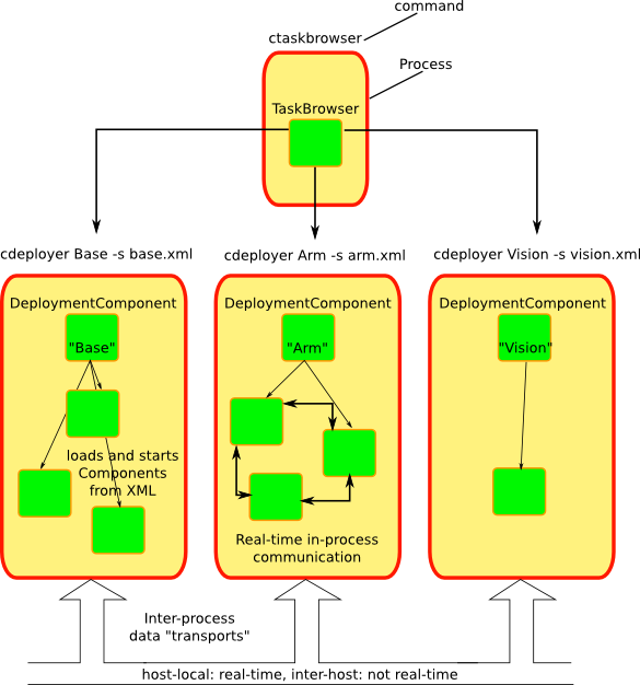
Components are loaded into the process by a deployer, which gets its configuration through an XML file. Communication between processes is transparant to the component, but your data must be known to Orocos (cfr 'typekits' and 'transports'). Most new users start with a single process however, using the 'deployer' application.
A component is a basic unit of functionality which executes one or more (real-time) programs in a single thread. The program can vary from a mere C/C++ function over a real-time program script to a real-time hierarchical state machine. The focus is completely on thread-safe time determinism. Meaning, that the system is free of priority-inversions, and all operations are lock-free. Real-time components can communicate with non real-time components (and vice verse) transparently.
| Note | |
|---|---|
In this manual, the words task and component are used as equal words, meaning a software component built using the C++ TaskContext class. |
The Orocos Component Model enables :
Lock free, thread-safe, inter-component communication in a single process.
Thread-safe, inter-process communication between (distributed) processes.
Communication between hard Real-Time and non Real-Time components.
Deterministic execution time during communication for the higher priority thread.
Synchronous and asynchronous communication between components.
Interfaces for run-time component introspection.
C++ class implementations and scripting interface for all the above.
The Scripting chapter gives more details about script syntax for state machines and programs.
| Important | |
|---|---|
Before you proceed, make sure you printed the Orocos Cheat Sheet and RTT Cheat Sheet ! They will definately guide you through this lengthy text. |
This section introduces tasks through the "hello world" application, for which you will create a component package using the orocreate-pkg command on the command line:
$ rosrun ocl orocreate-pkg HelloWorld # ... for ROS users
$ orocreate-pkg HelloWorld # ... for non-ROS users
In a properly configured installation, you'll be able to enter this directory and build your package right away:
$	cd HelloWorld
$ make
In case you are not using ROS to manage your packages, you also need to install your package:
$ make install
The way we interact with TaskContexts during development of an Orocos application is through the deployer . This application consists of the DeploymentComponent which is responsible for creating applications out of component libraries and the DeploymentComponent which is a powerful console tool which helps you to explore, execute and debug componentss in running programs.
The TaskBrowser uses the GNU readline library to easily enter commands to the tasks in your system. This means you can press TAB to complete your commands or press the up arrow to scroll through previous commands.
You can start the deployer in any directory like this:
$ deployer-gnulinux
or in a ROS environment:
$ rosrun ocl deployer-gnulinux
This is going to be your primary tool to explore the Orocos component model so get your seatbelts fastened!
Now let's start the HelloWorld application we just created with orocreate-pkg.
Create an 'helloworld.ops' Orocos Program Script (ops) file with these contents:
 require("print")        // necessary for 'print.ln'
 import("HelloWorld")    // 'HelloWorld' is a directory name to import

 print.ln("Script imported HelloWorld package:")
 displayComponentTypes() // Function of the DeploymentComponent

 loadComponent("Hello", "HelloWorld") // Creates a new component of type 'HelloWorld'
 print.ln("Script created Hello Component with period: " + Hello.getPeriod() )
and load it into the deployer using this command: $ deployer-gnulinux -s helloworld.ops -linfo This command imports the HelloWorld package and any component library in there. Then it creates a component with name "Hello". We call this a dynamic deployment, since the decision to create components is done at run-time.
You could also create your component in a C++ program. We call this static deployment, since the components are fixed at compilation time. The figure below illustrates this difference:
Figure 2.2. Dynamic vs static loading of components
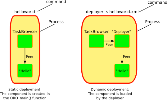
The 'helloworld' executable is a static deployment of one component in a process, which means it is hard-coded in the helloworld.cpp file. In contrast, using the deployer application allows you to load a component library dynamically.
The output of the deployer should be similar to what we show below. Finally, type cd Hello to start with the exercise.
0.000 [ Info   ][Logger] Real-time memory: 14096 bytes free of 20480 allocated.
0.000 [ Info   ][Logger] No RTT_COMPONENT_PATH set. Using default: .../rtt/install/lib/orocos
0.000 [ Info   ][Logger] plugin 'rtt' not loaded before.

...

0.046 [ Info   ][Logger] Loading Service or Plugin scripting in TaskContext Deployer
0.047 [ Info   ][Logger] Found complete interface of requested service 'scripting'
0.047 [ Info   ][Logger] Running Script helloworld.ops ...
0.050 [ Info   ][DeploymentComponent::import] Importing directory .../HelloWorld/lib/orocos/gnulinux ...
0.050 [ Info   ][DeploymentComponent::import] Loaded component type 'HelloWorld'
Script imported HelloWorld package:
I can create the following component types:
   HelloWorld
   OCL::ConsoleReporting
   OCL::FileReporting
   OCL::HMIConsoleOutput
   OCL::HelloWorld
   OCL::TcpReporting
   OCL::TimerComponent
   OCL::logging::Appender
   OCL::logging::FileAppender
   OCL::logging::LoggingService
   OCL::logging::OstreamAppender
   TaskContext
0.052 [ Info   ][Thread] Creating Thread for scheduler: 0
0.052 [ Info   ][Hello] Thread created with scheduler type '0', priority 0, cpu affinity 15 and period 0.
HelloWorld constructed !
0.052 [ Info   ][DeploymentComponent::loadComponent] Adding Hello as new peer:  OK.
Script created Hello Component with period: 0
0.053 [ Info   ][Thread] Creating Thread for scheduler: 0
0.053 [ Info   ][TaskBrowser] Thread created with scheduler type '0', priority 0, cpu affinity 15 and period 0.
   Switched to : Deployer
0.053 [ Info   ][Logger] Entering Task Deployer

  This console reader allows you to browse and manipulate TaskContexts.
  You can type in an operation, expression, create or change variables.
  (type 'help' for instructions and 'ls' for context info)
    TAB completion and HISTORY is available ('bash' like)

Deployer [S]> cd Hello
   Switched to : Hello
Hello [S]>
The first [ Info ] lines are printed by the Orocos Logger, which has been configured to display informative messages to console with the -linfo program option. Normally, only warnings or worse are displayed by Orocos. You can always watch the log file 'orocos.log' in the same directory to see all messages. After the [Log Level], the [Origin] of the message is printed, and finally the message itself. These messages leave a trace of what was going on in the main() function before the prompt appeared.
Depending on what you type, the TaskBrowser will act differently. The built-in commands cd, help, quit, ls etc, are seen as commands to the TaskBrowser itself, if you typed something else, it tries to execute your command according to the Orocos scripting language syntax.
Hello[R] > 1+1
   = 2
A component's interface consists of: Attributes and Properties, Operations, and Data Flow ports which are all public. The class TaskContext groups all these interfaces and serves as the basic building block of applications. A component developer 'builds' these interfaces using the instructions found in this manual.
To display the contents of the current component, type ls, and switch to one of the listed peers with cd, while cd .. takes you one peer back in history. We have two peers here: the Deployer and your component, Hello.
Hello [S]> ls

 Listing TaskContext Hello[S] :

 Configuration Properties: (none)

 Provided Interface:
  Attributes   : (none)
  Operations   : activate cleanup configure error getCpuAffinity getPeriod inFatalError inRunTimeError isActive isConfigured isRunning setCpuAffinity setPeriod start stop trigger update

 Data Flow Ports: (none)

 Services:
(none)

 Requires Operations :  (none)
 Requests Services   :  (none)

 Peers        : (none)
Hello [S]>
| Note | |
|---|---|
To get a quick overview of the commands, type help. |
The first line shows the status between square brackets. The [S] here means that the component is in the stopped state. Other states can be 'R' - Running, 'U' - Unconfigured, 'E' - run-time Error, 'F' - Fatal error, 'X' - C++ eXception in user code.
First you get a list of the Properties and Attributes (alphabetical) of the current component. Properties are meant for configuration and can be written to disk. Attributes export a C++ class value to the interface, to be usable by scripts or for debugging and are not persistent.
Next, the operations of this component are listed: each component has some universal functions like activate, start, getPeriod etc.
You can see that the component is pretty empty: no data flow ports, services or peers. We will add some of these right away.
To get an overview of the Task's interface, you can use the help command, for example help this or help this.activate or just short: help activate
Hello [R]> help this

Printing Interface of 'Hello' :

 activate( ) : bool
   Activate the Execution Engine of this TaskContext (= events and commands).
 cleanup( ) : bool
   Reset this TaskContext to the PreOperational state (write properties etc).
...
   Stop the Execution Engine of this TaskContext.

Hello [R]> help getPeriod
 getPeriod( ) : double
Get the configured execution period. -1.0: no thread associated, 0.0: non periodic, > 0.0: the period.

Hello [R]>
Now we get more details about the operations registered in the public interface. We see now that the getPeriod operations takes no arguments You can invoke each operation right away.
Hello [R]> getPeriod()
 = 0
Operations are called directly and the TaskBrowser prints the result. The return value of getPeriod() was a double, which is 0. This works just like calling a 'C' function. You can express calling explicitly by writing: getPeriod.call().
When an operation is sent to the Hello component, another thread will execute it on behalf of the sender. Each sent method returns a SendHandle object.
Hello [R]> getPeriod.send()
 = (unknown_t)
The returned SendHandle must be stored in a SendHandle attribute to be useful:
Hello [R]> var SendHandle sh
Hello [R]> sh = getPeriod.send()
 = true
Hello [R]> sh.collectIfDone( ret )
 = SendSuccess
Hello [R]> ret
 = 0
SendHandles are further explained down the document. They are not required understanding for a first discovery of the Orocos world.
Besides calling or sending component methods, you can alter the attributes of any task, program or state machine. The TaskBrowser will confirm validity of the assignment with the contents of the variable. Since Hello doesn't have any attributes, we create one dynamically:
Hello [R]> var string the_attribute = "HelloWorld"
Hello [R]> the_attribute
 = Hello World
Hello [R]> the_attribute = "Veni Vidi Vici !"
 = "Veni Vidi Vici !"
Hello [R]> the_attribute
 = Veni Vidi Vici !
The Data Ports allow seamless communication of calculation or measurement results between components. Adding and using ports is described in Section 3.3, “Data Flow Ports”.
Last but not least, hitting TAB twice, will show you a list of possible completions, such as peers, services or methods.
TAB completion works even across peers, such that you can type a TAB completed command to another peer than the current peer.
In order to quit the TaskBrowser, enter quit:
 Hello [R]> quit

1575.720 [ Info   ][ExecutionEngine::setActivity] Hello is disconnected from its activity.
1575.741 [ Info   ][Logger] Orocos Logging Deactivated.
The TaskBrowser Component is application independent, so that your end user-application might need a more suitable interface. However, for testing and inspecting what is happening inside your real-time programs, it is a very useful tool. The next sections show how you can add properties, methods etc to a TaskContext.
| Note | |
|---|---|
If you want a more in-depth tutorial, see the rtt-exercises package which covers each aspect also shown in this manual. |
Components are implemented by subclassing the TaskContext class. It is useful speaking of a context because it defines the context in which an activity (a program) operates. It defines the interface of the component, its properties, its peer components and uses its ExecutionEngine to execute its programs and to process asynchronous messages.
This section walks you through the definition of an example component in order to show you how you could build your own component.
A new component is constructed as :
  #include <rtt/TaskContext.hpp>
  #include <rtt/Component.hpp>

  // we assume this is done in all the following code listings :
  using namespace RTT;

  class MyTask : public TaskContext
  {
  public:
       ATask(const std::string& name) : public TaskContext(name) {}
  };

  // from Component.hpp:
  OCL_CREATE_COMPONENT( MyTask );
The constructor argument is the (unique) name of the component. You should create the component template and the CMakeLists.txt file using the orocreate-pkg program such that this compiles right away as in the HelloWorld example above:
$ orocreate-pkg mytask
You can load this package in a deployer by using the import command at the TaskBrowser prompt and verify that it contains components using displayComponentTypes() in the TaskBrowser. After import, loadComponent("the_task","MyTask") loads a new component instance into the process:
      $ deployer-gnulinux
      ...
			Deployer [S]> import("mytask")    // 'mytask' is a directory name to import
			Deployer [S]> displayComponentTypes() // lists 'MyTask' among others
			...
			MyTask
			...
			Deployer [S]> loadComponent("the_task", "MyTask") // Creates a new component of type 'MyTask'
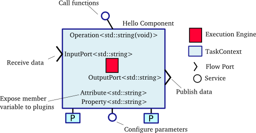
Figure 2.4. Schematic Overview of a TaskContext
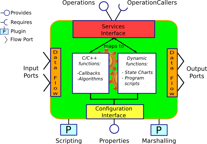
The component offers services through operations, and requests them through operation callers. The Data Flow is the propagation of data from one task to another, where one producer can have multiple consumers and the other way around.
The beating hart of the component is its Execution Engine will check for new messages in it's queue and execute programs which are running in the task. When a TaskContext is created, the ExecutionEngine is always running. The complete state flow of a TaskContext is shown in Figure 2.5, “ TaskContext State Diagram ”. You can add code in the TaskContext by implementing *Hook() functions, which will be called by the ExecutionEngine when it is in a certain state or transitioning between states.
Figure 2.5. TaskContext State Diagram
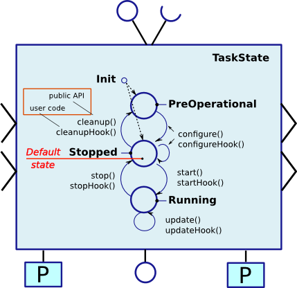
During creation, a component is in the
Init state. When constructed, it
enters the PreOperational or
Stopped (default) state. If it enters
the PreOperational state after construction, it requires
an additional configure() call before
it can be start()'ed. The figure
shows that for each API function, a user 'hook' is
available.
The first section goes into detail on how to use these hooks.
The user application code is filled in by inheriting from the TaskContext and implementing the 'Hook' functions. There are five such functions which are called when a TaskContext's state changes.
The user may insert his configuration-time setup/cleanup code in the
configureHook() (read XML, print status
messages etc.) and cleanupHook() (write
XML, free resources etc.).
The run-time (or: real-time) application code belongs in the
startHook(),
updateHook() and
stopHook() functions.
class MyTask
    : public TaskContext
  {
  public:
       MyTask(std::string name)
         : TaskContext(name)
       {
          // see later on what to put here.
       }

       /**
        * This function is for the configuration code.
        * Return false to abort configuration.
        */
       bool configureHook() {
          // ...
          return true;
       }

       /**
        * This function is for the application's start up code.
        * Return false to abort start up.
        */
       bool startHook() {
          // ...
          return true;
       }

       /**
        * This function is called by the Execution Engine.
        */
       void updateHook() {
          // Your component's algorithm/code goes in here.
       }

       /**
        * This function is called when the task is stopped.
        */
       void stopHook() {
          // Your stop code after last updateHook()
       }

       /**
        * This function is called when the task is being deconfigured.
        */
       void cleanupHook() {
          // Your configuration cleanup code
       }
};| Important | |
|---|---|
By default, the TaskContext enters the
|
If you want to force the user to call configure() of your TaskContext, set the TaskState in your constructor as such:
class MyTask
    : public TaskContext
  {
  public:
       MyTask(std::string name)
         : TaskContext(name, PreOperational) // demand configure() call.
       {
          //...
       }
  };
When configure() is called, the
configureHook() (which you
must implement!) is executed and must return
false if it failed. The TaskContext drops to the
PreOperational state in that case.
When configureHook() succeeds, the
TaskContext enters the Stopped state
and is ready to run.
A TaskContext in the Stopped state
(Figure 2.5, “
TaskContext State Diagram
”)
may be start()'ed upon which
startHook() is called once and may abort
the start up sequence by returning false. If true, it enters the
Running state and
updateHook() is called (a)periodically by
the ExecutionEngine, see below. When the task is
stop()'ed, stopHook()
is called after the last updateHook() and
the TaskContext enters the Stopped state
again. Finally, by calling cleanup(), the
cleanupHook() is called and the TaskContext
enters the PreOperational state.
The functionality of a component, i.e. its algorithm, is executed
by its internal Execution Engine. To run a TaskContext, you
need to use one of the
ActivityInterface classes from the
RTT, most likely Activity. This
relation is shown in Figure 2.6, “
Executing a TaskContext
”.
The Activity class allocates a thread which executes the
Execution Engine. The chosen
Activity object will run
the Execution Engine, which will in turn call the
application's hooks above. When created, the TaskContext is assigned
the Activity by default.
It offers an internal thread which can receive messagse
and process events but is not periodicly executing
updateHook().
Figure 2.6. Executing a TaskContext
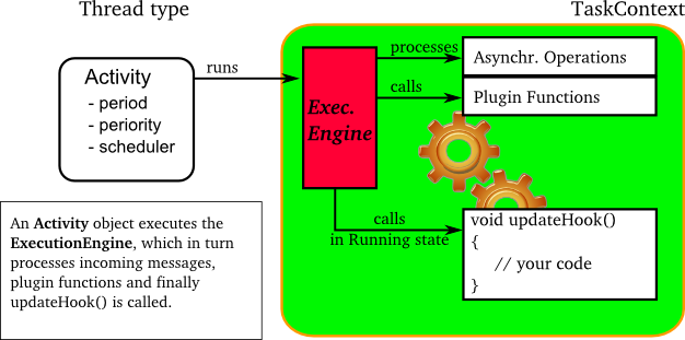
You can make a TaskContext 'active' by creating an Activity object which executes its Execution Engine.
A common task in control is executing an algorithm periodically. This is done by attaching an activity to the Execution Engine which has a periodic execution time set.
  #include <rtt/Activity.hpp>

  using namespace RTT;

  TaskContext* a_task = new MyTask("the_task");
  // Set a periodic activity with priority=5, period=1000Hz
  a_task->setActivity( new Activity( 5, 0.001 ));
  // ... start the component:
  a_task->start();
  // ...
  a_task->stop();
Which will run the Execution Engine of "ATask" with a
frequency of 1kHz. This is the frequency at which state
machines are evaluated, program steps taken, methods and
messages are accepted and executed and the application code in
updateHook() is run. Normally this activity
is always running, but you can stop and start it too.
You don't need to create a new Activity if you want to switch
to periodic execution, you can also use the setPeriod
function:
  // In your TaskContext's configureHook():
  bool configureHook() {
      return this->setPeriod(0.001); // set to 1000Hz execution mode.
  }
An updateHook() function of a periodic
task could look like:
  class MyTask
    : public TaskContext
  {
  public:
       // ...

       /**
        * This function is periodically called.
        */
       void updateHook() {
          // Your algorithm for periodic execution goes inhere
          double result;
          if ( inPort.read(result) == NewData )
              outPort.write( result * 2.0 ); // only write if new data arrived.
       }

  };
You can find more detailed information in Section 2, “Activities” in the CoreLib reference.
A TaskContext is run by default by a non periodic RTT:Activity object. This
is useful when updateHook() only needs
to process data when it arrives on a port or must wait on
network connections or does any other blocking operation.
Upon start(), the Execution Engine waits for new methods or data to
come in to be executed. Each time such an event happens, the user's
application code (updateHook()) is called
after the Execution Engine did its work.
An updateHook() function of a non periodic
task could look like:
  class MyTask
    : public TaskContext
  {
  public:
       // ...

       /**
        * This function is only called by the Execution Engine
        * when 'trigger()' is called or an event or command arrives.
        */
       void updateHook() {
            // Your blocking algorithm goes inhere
            char* data;
            double timeout = 0.02; // 20ms
            int rv = my_socket_read(data, timeout);

            if (rv == 0) {
               // process data
               this->stateUpdate(data);
            }

            // This is special for non periodic activities, it makes
            // the TaskContext call updateHook() again after
            // commands and events are processed.
            this->getActivity()->trigger();
       }

};| Warning | |
|---|---|
Non periodic activities should be used with care and with much thought in combination with scripts (see later). The ExecutionEngine will do absolutely nothing if no asynchronous methods or asynchronous events or no trigger comes in. This may lead to surprising 'bugs' when program scripts or state machine scripts are executed, as they will only progress upon these events and seem to be stalled otherwise. |
You can find more detailed information in Section 2, “Activities” in the CoreLib reference.
| Purpose | |
|---|---|
A component has ports in order to send or receive a stream of data. The algorithm writes Output ports to publish data to other components, while input ports allow an algorithm to receive data from other components. A component can be woken up if data arrives at one or more input ports or it can 'poll' for new data on its input ports. Reading and writing data ports is always real-time and thread-safe, on the condition that copying your data (i.e. your operator= ) is as well. |
Each component defines its data exchange ports and connections transmit data from one port to another. A Port is defined by a name, unique within that component, the data type it wants to exchange and if its for reading (Input) or writing (Output) data samples. Finally, you can opt that new data on selected Input ports wake up your task. The example below shows all these possibilities.
Each connection between an Output port and an Input port can be tuned for your setup: buffering of data, thread-safety and initialisation of the connection are parameters provided by the user when the connection is created. We call these Connection Policies and use the ConnPolicy object when creating the connection between ports.
Figure 2.7. Data flow ports are connected with a connection policy
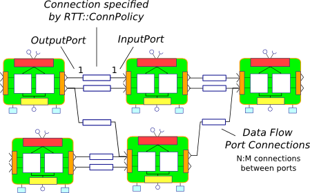
This figure shows that input and output ports can be connected in an N:M way. See Section 4.2, “Setting up the Data Flow” on how to connect ports and which connection policy to choose.
The data flow implementation can pass on any data type 'X', given that its class provides:
A default constructor: X::X()
An assignment operator: const X& X::operator=(const X& )
For real-time data transfer (see also Section 3.3.3, “Guaranteeing Real-Time data flow”) the operator= must be real-time when assigning equal sized objects. When assigning not equal sized objects, your operator= should free the memory and allocate enough room for the new size.
In addition, if you want to send your data out of your process to another process or host, it will additionally need:
Registration of 'X' with the type system (see the manual about Typekits)
A transport for the data type registered with the type system (see the transport (ROS,CORBA,MQueue,...) documentation)
The standard C++ and std::vector<double> data types are already included in the RTT library for real-time transfer and out of process transport.
Any kind of data can be exchanged (also user defined C/C++ types) but for readability, only the 'double' C type is used here.
  #include <rtt/Port.hpp>
  using namespace RTT;

  class MyTask
    : public TaskContext
  {
    // Input port: We'll let this one wake up our thread
    InputPort<double> evPort;

    // Input port: We will poll this one
    InputPort<double> inPort;

    // Output ports are allways 'send and forget'
    OutputPort<double> outPort;
  public:
    // ...
    MyTask(std::string name)
      : TaskContext(name)
    {
       // an 'EventPort' is an InputPort which wakes our task up when data arrives.
       this->ports()->addEventPort( "evPort", evPort ).doc( "Input Port that raises an event." );

       // These ports do not wake up our task
       this->ports()->addPort( "inPort", inPort ).doc( "Input Port that does *not* raise an event." );
       this->ports()->addPort( "outPort", outPort ).doc( "Output Port, here write our data to." );

       // more additions to follow, see below
     }

     // ...
  };
The example starts with declaring all the ports of MyTask. A template parameter '<double>' specifies the type of data the task wants to exchange through that port. Logically, if input and output are to be connected, they must agree on this type. The name is given in the addPort() function. This name can be used to 'match' ports between connected tasks ( using 'connectPorts', see Section 4, “Connecting Services” ), but it is possible and preferred to connect Ports with different names using the Orocos deployer.
There are two ways to add a port to the TaskContext interface:
using addPort()
or addEventPort(). In the latter case,
new data arriving on the port will wake up ('trigger') the
activity of our TaskContext and updateHook() get's executed.
| Note | |
|---|---|
Only InputPort can be added as EventPort and will cause your component to be triggered (ie wake up and call updateHook). |
The data flow implementation is written towards hard real-time data transfer, if the data type allows it. Simple data types, like a double or struct with only data which can be copied without causing memory allocations work out of the box. No special measures must be taken and the port is immediately ready to use.
If however, your type is more complex, like a std::vector or other dynamically sized object, additional setup steps must be done. First, the type must guarantee that its operator=() is real-time in case two equal-sized objects are used. Second, before sending the first data to the port, a properly sized data sample must be given to the output port. An example:
  OutputPort<std::vector<double> > myport("name");

  // create an example data sample of size 10:
  std::vector<double> example(10, 0.0);

  // show it to the port (this is a not real-time operation):
  myport.setDataSample( example );

  // Now we are fine ! All items sent into the port of size 10 or less will
  // be passed on in hard real-time.
  myport.write( example ); // hard real-time.
setDataSample does not actually send the data to all receivers, it just uses this sample to initiate the connection, such that any subsequent writes to the port with a similar sample will be hard real-time. If you omit this call, data transfer will proceed, but the RTT makes no guarantees about real-timeness of the transfer.
The same procedure holds if you use transports to send data to other processes or hosts. However, it will be the transport protocol that determines if the transfer is real-time or not. For example, CORBA transports are not hard real-time, while MQueue transports are.
The Data Flow interface is used by your task from within
the program scripts or its updateHook()
method. Logically the script or method reads the inbound
data, calculates something and writes the outbound data.
  #include <rtt/Port.hpp>
  using namespace RTT;

  class MyTask
    : public TaskContext
  {
     // ...Constructor sets up Ports, see above.

     bool startHook() {
       // Check validity of (all) Ports:
       if ( !inPort.connected() ) {
          // No connection was made, can't do my job !
          return false;
       }
       if ( !outPort.connected() ) {
          // ... not necessarily an error, a connection may be
          // made while we are running.
       }
       return true;
     }

     /**
      * Note: use updateHook(const std::vector<PortInterface*>&)
      * instead for having information about the updated event
      * driven ports.
      */
     void updateHook() {

       double val = 0.0;

       // Possible return values are: NoData, OldData and NewData.
       if ( inPort.read(val) == RTT::NewData ) {
         // update val...
         outPort.write( val );
       }
     }
     // ...
  };
It is wise to check in the startHook()
( or earlier: in configureHook() )
function if all necessary ports are
connected(). At this point, the task
start up can still be aborted by returning false. Otherwise,
a write to an unconnected output port will be discarded,
while a read from an unconnected input port returns NoData.
When a Port is added, it becomes available to the Orocos scripting system such that (part of) the calculation can happen in a script. Also, the TaskBrowser can then be used to inspect the contents of the DataFlow on-line.
| Note | |
|---|---|
In scripting, it is currently not yet possible to know which event port woke your task up. |
A small program script could be loaded into MyTask with the following contents:
  program MyControlProgram {
    var double the_K  = K        // read task property, see later.
    var double setp_d

    while ( true ) {
      if ( SetPoint_X.read( setp_d ) != NoData ) {   // read Input Port
        var double in_d = 0.0;
        Data_R.read( in_d )             // read Input Port
        var double out_d = (setp_d - in_d) * the_K  // Calculate
        Data_W.write( out_d )          // write Data Port
      }
      yield       // this is a 'yield' point to avoid inifinite spinning.
    }
  }
The program "MyControlProgram" starts with declaring two variables and reading the task's Property 'K'. Then it goes into an endless loop, trying to Pop a set point value from the "SetPoint_X" Port. If that succeeds (new or old data present) the "Data_R" Port is read and a simple calculation is done. The result is written to the "Data_W" OutputPort and can now be read by the other end(s). Alternatively, the result may be directly used by the Task in order to write it to a device or any non-task object. You can use methods (below) to send data from scripts back to the C++ implementation.
Remark that the program is executed within the thread of the component.
In order to avoid the endless loop, a 'wait' point
must be present. The "yield" command inserts such a
wait point and is part of the Scripting syntax. If you plan
to use Scripting state machines, such a
while(true) loop (and hence wait point)
is not necessary. See the Scripting Manual for a full
overview of the syntax.
| Purpose | |
|---|---|
A task's operations define which functions a component offers. Operations are grouped in 'services', much like C++ class methods are grouped in classes. OperationCallers are helper objects for calling operations. |
Operations are C/C++ functions that can be used in scripting or can be called from another process or accross a network. They take arguments and return a value. The return value can in return be used as an argument for other Operations or stored in a variable.
To add a C/C++ function to the operation interface, you
only need to register it with addOperation(),
defined in Service.
  #include <rtt/Operation.hpp>
  using namespace RTT;

  class MyTask
    : public TaskContext
  {
    public:
    void reset() { ... }
    string getName() const { ... }
    double changeParameter(double f) { ... }
    // ...

    MyTask(std::string name)
      : TaskContext(name),
    {
       // Add the method objects to the method interface:
       this->addOperation( "reset",  &MyTask::reset, this, OwnThread)
                                   .doc("Reset the system.");
       this->addOperation( "getName", &MyTask::getName, this, ClientThread)
                                   .doc("Read out the name of the system.");
       this->addOperation( "changeParameter", &MyTask::changeParameter, this, OwnThread)
                                   .doc("Change a parameter, return the old value.")
                                   .arg("New Value", "The new value for the parameter.");

       // more additions to follow, see below
     }
     // ...
  };
In the above example, we wish to add 3 functions to the method interface: reset, getName and changeParameter. You need to pass the name of the function, address (function pointer) of this function and the object on which it must be called (this) to addOperation. Optionally, you may document the operation with .doc("...") and each argument with a .arg() call.
Using this mechanism, any method of any class can be added to a task's method interface, not just functions of a TaskContext You can also add plain C functions, just omit the this pointer.
As the last argument to addOperation, a flag can be passed which can be OwnThread or ClientThread. This allows the component implementer to choose if the operation, when called, is executed in the thread of the ExecutionEngine, or in the thread of the caller (i.e. the Client). This choice is hidden from the user of our operations. It allows us to choose who gets the burden of the execution of the function, but also allows to synchronize operation calls with the execution of updateHook(). Summarized in a table:
Table 2.1. Execution Types
| ExecutionType | Requires locks in your component? | Executed at priority of | Examples |
|---|---|---|---|
| ClientThread | Yes. For any data shared between the ClientThread-tagged operation and updateHook() or other operations. | Caller thread |
|
| OwnThread | No. Every OwnThread-tagged operation and updateHook() is executed in the thread of the component. | Component thread. |
|
The choice of this type is completely up to the implementor of the component and can be made independently of how it will be used by its clients. Clients can indicate the same choice indepenently: they can Call or Send an operation. This is explained in the next two sections.
Operations are added to the TaskContext's inteface. To call an operation from another component, you need a OperationCaller object to do the work for you. It allows to modes:
calling the operation, in which case you block until the operation returns its value
sending the operation, in which case you get a SendHandle back which allows you to follow its status and collect the results.
One OperationCaller object always offers both choices, and they can be used both interweaved, as far as the allocation scheme allows it. See Section 3.4.4, “Executing methods in real-time.”. Calling is used by default if you don't specify which mode you want to use.
Each OperationCaller object is templated with the function signature of the operation you wish to call. For example
void(int,double)
which is the signature of a
function returning 'void' and having two arguments: an
'int' and a 'double', for example, void foo(int
i, double d);.
To setup a OperationCaller object, you need a pointer to a TaskContext object, for example using the 'getPeer()' class function. Then you provide the name with which the operation was registered during 'addOperation':
  // create a method:
  TaskContext* a_task_ptr = getPeer("ATask");
  OperationCaller<void(void)> my_reset_meth
       = a_task_ptr->getOperation("reset"); // void reset(void)

  // Call 'reset' of a_task:
  reset_meth();
If you wanted to send the same reset operation, you had written:
  // Send 'reset' of a_task:
  SendHandle<void(void)> handle = reset_meth.send();
A send() always returns a SendHandle object which offers three
methods: collect(),
collectIfDone() and ret().
All three come in two forms: with arguments or without arguments.
The form without arguments can be used if you are only interested in
the return values of these functions. collect() and collectIfDone()
return a SendStatus, ret() returns the return value of the operation.
SendStatus is an enum of SendSuccess, SendNotReady or SendFailure.
Code says it all:
  // Send 'reset' of a_task:
  SendHandle<void(void)> handle = reset_meth.send();

  // polling for reset() to complete:
  while (handle.collectIfDone() == SendNotReady )
      sleep(1);

  // blocking for reset() to complete:
  handle = reset_meth.send();
  SendStatus ss = handle.collect();
  if (ss != SendSuccess) {
      cout << "Execution of reset failed." << endl;
  }

  // retrieving the return value is not possible for a void(void) method.
Next we move on to methods with arguments and return values by using the getName and changeParameter operations:
  // used to hold the return value of getName:
  string name;
  OperationCaller<string(void)> name_meth =
    a_task_ptr->getOperation("getName"); // string getName(void)

  // Call 'getName' of a_task:
  name = name_meth();
  // Equivalent to:
  name = name_meth.call();

  cout << "Name was: " << name << endl;

  // Send 'getName' to a_task:
  SendHandle<string(void)> nhandle = name.send();

  // collect takes the return value of getName() as first argument and fills it in:
  SendStatus ss = nhandle.collect(name);
  if (ss == SendSuccess) {
    cout << "Name was: " << name << endl;
  }

  assert( name == nhandle.ret() ); // ret() returns the same as getName() returned.

  // hold return value of changeParameter:
  double oldvalue;
  OperationCaller<double(double)> mychange =
      a_task_ptr->getOperation("changeParameter"); // double changeParameter(double)

  // Call 'changeParameter' of a_task with argument '1.0'
  oldvalue = mychange( 1.0 );
  // Equivalent to:
  oldvalue = mychange.call( 1.0 );

  // Send 'changeParameter' to a_task:
  SendHandle<double(double)> chandle = changeParameter.send( 2.0 )

  SendStatus ss = chandle.collectIfDone( oldvalue );
  if (ss == SendSuccess) {
      cout << "Oldvalue was: " << oldvalue << endl;
  }
Up to 4 arguments can be given to send or call. If the signature of the OperationCaller was not correct, the method invocation will be throw. One can check validity of a method object with the 'ready()' function:
  OperationCaller<double(double)> mychange = ...;
  assert( mychange.ready() );
The syntax in scripts is the same as in C++:
 // call:
  var double oldvalue
  ATask.changeParameter( 0.1 )
  // or :
  set oldvalue = ATask.changeParameter( 0.1 ) // store return value

  // send:
  var SendHandle handle;
  var SendStatus ss;
  handle = ATask.changeParameter.send( 2.0 );

  // collect non-blocking:
  while ( handle.collectIfDone( oldvalue ) )
     yield // see text below.

  // collect blocking:
  handle.collect( oldvalue ); // see text below.
There is an important difference between collect() and collectIfDone() in scripts. collect() will block your whole script, so also other scripts executed in the ExecutionEngine and updateHook(). The only exception is that incomming operations are still processed, such that call-backs are allowed. For example: if ATask.changeParameter( 0.1 ) does in turn a send on your component, this will be processed such that no dead-lock occurs.
If you do not wish to block unconditionally on the completion of changeParameter(), you can poll with collectIfDone(). Each time the poll fails, you issue a yield (in RTT 1.x this was 'do nothing'). Yield causes temporary suspension of your script, such that other scripts and updateHook() get a chance to run. In the next trigger of your component, the program resumes and the while loop checks the collectIfDone() statement again.
Considering all the combinations above, 4 cases can occur:
Table 2.2. Call/Send and ClientThread/OwnThread Combinations
| OperationCaller-v \ Operation-> | ClientThread | OwnThread |
|---|---|---|
| Call | Executed directly by the thread that does the call() | Executed by the ExecutionEngine of the receiving component. |
| Send | Executed by the GlobalExecutionEngine. See text below. | Executed by the ExecutionEngine of the receiving component. |
This matrix shows a special case: when the client does a send() and the component defined the operation as 'ClientThread', someone else needs to execute it. That's the job of the GlobalExecutionEngine. Since no thread wishes to carry the burden of executing this function, the GlobalExecutionEngine, which runs with the lowest priority thread in the system, picks it up.
Calling or sending a method has a cost in terms of memory. The implementations needs to allocate memory to collect the return values when a send or call is done. There are two ways to claim memory: by using a real-time memory allocator or by setting a fixed amount in the OperationCaller object in advance. The default is using the real-time memory allocator. For mission critical code, you can override this with a reserved amount, which will be guaranteed always available for that object.
(to be completed).
The arguments can be of any class type and type qualifier (const, &, *,...). However, to be compatible with inter-process communication or the Orocos Scripting variables, it is best to follow the following guidelines :
Table 2.3. Operation Return & Argument Types
| C++ Type | In C++ functions passed by | Maps to Parser variable type |
|---|---|---|
| Primitive C types : double, int, bool, char | value or reference | double, int, bool, char |
| C++ Container types : std::string, std::vector<double> | (const) & | string, array |
| Orocos Fixed Container types : RTT::Double6D, KDL::[Frame | Rotation | Twist | ... ] | (const) & | double6d, frame, rotation, twist, ... |
Summarised, every non-class argument is best passed by value, and every class type is best passed by const reference. The parser does handle references (&) in the arguments or return type as well.
| Purpose | |
|---|---|
A task's properties are intended to configure and tune a task with certain values. Properties have the advantage of being writable to an XML format, hence can store 'persistent' state. For example, a control parameter. Attributes reflect a C++ class variable in the interface and can be read and written during run-time by a program script, having the same data as if it was a C++ function. Reading and writing properties and attributes is real-time but not thread-safe and should for a running component be limited to the task's own activity. |
A TaskContext may have any number of attributes or properties, of any type. They can be used by programs in the TaskContext to get (and set) configuration data. The task allows to store any C++ value type and also knows how to handle Property objects. Attributes are plain variables, while properties can be written to and updated from an XML file.
An attribute can be added in the comonent's interface (ConfigurationInterface) like this :
  #include <rtt/Property.hpp>
  #include <rtt/Attribute.hpp>

  class MyTask
    : public TaskContext
  {
     // we will expose these:
     bool aflag;
     int max;

     double pi;

     std::string param;
     double value;
  public:
    // ...
    MyTask(std::string name)
      : TaskContext(name),
        param("The String"),
        value( 1.23 ),
        aflag(false), max(5), pi(3.14)
    {
       // other code here...

       // attributes and constants don't take a .doc() description.
       this->addAttribute( "aflag", aflag );
       this->addAttribute( "max", max );

       this->addConstant( "pi", pi );

       this->addProperty( "Param", param ).doc("Param Description");
       this->addProperty( "Palue", value ).doc("Value Description");
     }
     // ...
  };
Which aliases an attribute of type bool and int, name 'aflag' and 'max' and initial value of false and 5 to the task's interface. A constant alias 'pi' is added as well. These methods return false if an attribute with that name already exists. Adding a Property is also straightforward. The property is added in a PropertyBag.
An attribute is used in your C++ code transparantly. For properties, you need their set() and get() methods to write and read them.
A external task can access attributes through an Attribute object and the getValue method:
  Attribute<bool> the_flag = a_task->getValue("aflag");
  assert( the_flag.ready() );

  bool result = the_flag.get();
  assert( result == false );

  Attribute<int> the_max = a_task->attributes()->getAttribute("max");
  assert( the_max.ready() );
  the_max.set( 10 );
  assert( the_max.get() == 10 );
The attributes 'the_flag' and 'the_max' are mirrors of the original attributes of the task.
See also Section 6, “Properties” in the Orocos CoreLib reference.
A program script can access the above attributes simply by naming them:
  // a program in "ATask" does :
  var double pi2 = pi * 2.
  var int    myMax = 3
  set max = myMax

  set Param = "B Value"
  // an external (peer task) program does :
  var double pi2 = ATask.pi * 2.
  var int    myMax = 3
  set ATask.max = myMax
When trying to assign a value to a constant, the script parser will throw an exception, thus before the program is run.
| Important | |
|---|---|
The same restrictions of Section 3.4.5, “Operation Argument and Return Types” hold for the attribute types, when you want to access them from program scripts. |
See also Section 5, “Attributes” in the Orocos CoreLib reference.
See Section 6.1, “Task Property Configuration and XML format” for storing and loading the Properties to and from files, in order to store a TaskContext's state.
In addition to the PreOperational,
Stopped and Running
TaskContext states, you can use two additional states for more
advanced component behaviour: the Exception, FatalError
and the RunTimeError states. The first two are shown in
Figure 2.8, “
Extended TaskContext State Diagram
”.
Figure 2.8. Extended TaskContext State Diagram
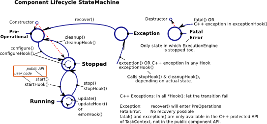
This figure shows the extended state diagram of a
TaskContext. This is Figure 2.5, “
TaskContext State Diagram
”
extended with two more states: Exception
and FatalError.
The FatalError state is entered whenever
the TaskContext's fatal() function is
called, and indicates that an unrecoverable error occured.
The ExecutionEngine is immediately
stopped and no more functions are called. This state can
not be left and the only next step is destruction of the component
(hence 'Fatal').
When an exception happens in your code, the Exception state
is entered. Depending on the TaskState, stopHook() and cleanupHook()
will be called to give a chance to cleanup. This state is recoverable
with the recover() function which drops your
component back to the PreOperational state,
from which it needs to be configured again.
It is possible that non-fatal run-time errors occur which
may require user action on one hand, but do not prevent
the component from performing it's task, or allow degraded
performance.
Therefor, in the Running state, one can
make a transition to theRunTimeError
sub-state by calling error(). See
Figure 2.9, “
Possible Run-Time failure.
”.
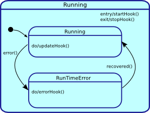
When the application code calls error(),
the RunTimeError state is entered and
errorHook() is executed instead of
updateHook(). If at some moment the
component detects that it can resume normal operation, it
calls the recover() function, which
leads to the Running state again and in the next iteration,
updateHook() is called again.
Here is a very simple use case, a TaskContext communicates over a socket with a remote device. Normally, we get a data packet every 10ms, but sometimes one may be missing. When we don't receive 5 packets in a row, we signal this as a run time error. From the moment packets come in again we go back to the run state. Now if the data we get is corrupt, we go into fatal error mode, as we have no idea what the current state of the remote device is, and shouldn't be updating our state, as no one can rely on the correct functioning of the TaskContext.
Here's the pseudo code:
 class MyComponent : public TaskContext
 {
       int faults;
 public:
       MyComponent(const std::string &name)
         : TaskContext(name), faults(0)
       {}

 protected:
       // Read data from a buffer.
       // If ok, process data. When to many faults occur,
       // trigger a runtime error.
       void updateHook()
       {
            Data_t data;
            FlowStatus rv = input.read( data );
            if ( rv == NewData ) {
               this->stateUpdate(data);
               faults = 0;
               this->recover(); // may be an external supervisor calls this instead.
            } else {
               faults++;
               if (faults > 4)
                   this->error();
            }

       }

       // Called instead of updateHook() when in runtime error state.
       void errorHook()
       {
            this->updateHook(); // just call updateHook anyway.
       }

       // Called by updateHook()
       void stateUpdate(Data_t data)
       {
            // Check for corrupt data
            if ( checkData(data) == -1 ) {
                 this->fatalError(); // we will enter the FatalError state.
            } else {
                 // data is ok: update internal state...
            }
       }
 };
When you want to discard the 'error' state of the component, call mycomp.recover(). If your component went into FatalError, call mycomp.reset() and mycomp.start() again for processing updateHook() again.
A Real-Time system exists of multiple concurrent tasks which must communicate to each other. TaskContext can be connected to each other such that they can use each other's Services.
| Note | |
|---|---|
The |
We call connected TaskContexts "Peers" because there is no implied
hierarchy. A connection from one TaskContext to its
Peer can be uni- or bi-directional. In a uni-directional connection (addPeer ),
only one peer can use the services of the other, while
in a bi-directional connection (connectPeers), both can use
each others services.
This allows to build strictly hierarchical topological
networks as well as complete flat or circular networks or any
kind of mixed network.
Peers are connected as such (hasPeer takes a string
argument ):
  // bi-directional :
  connectPeers( &a_task, &b_task );
  assert( a_task.hasPeer( &b_task.getName() )
          & b_task.hasPeer( &a_task.getName() ) );

  // uni-directional :
  a_task.addPeer( &c_task );
  assert( a_task.hasPeer( &c_task.getName() )
          & ! c_task.hasPeer( &a_task.getName() ) );

  // Access the interface of a Peer:
  OperationCaller<bool(void)> m = a_task.getPeer( "CTask" )->getOperation("aOperationCaller");
  // etc. See interface usage in previous sections.
Both connectPeers and addPeer
allow scripts or C++ code to use the interface of a connected Peer. connectPeers
does this connection in both directions.
From within a program script, peers can be accessed by merely prefixing their name to the member you want to access. A program within "ATask" could access its peers as such :
 // Script:
  var bool result = CTask.aOperation()
The peer connection graph can be traversed at arbitrary depth. Thus you can access your peer's peers.
| Note | |
|---|---|
In typical applications, the DeploymentComponent ('deployer') will form connections between ports using a program script or XML file. The manual method described below is not needed in that case. |
Data Flow between TaskContexts can be setup by using connectPorts.
The direction of the data flow is imposed by the input/output direction of
the ports. The connectPorts(TaskContext* A, TaskContext* B) function
creates a connection between TaskContext ports when both ports
have the same name and type. It will never disconnect existing connections
and only tries to add ports to existing connections or create new
connections. The disadvantage of this approach is that you can not specify
connection policies.
Instead of calling connectPorts, one may connect individual ports,
such that different named ports can be connected and a connection policy can be set.
Suppose that Task A has a
port a_port, Task B a b_port and Task C a c_port (all are of type PortInterface&). Then
connections are made as follows:
  // Create a connection with a buffer of size 10:
  ConnPolicy policy = RTT::ConnPolicy::buffer(10);
  a_port.connectTo( &b_port, policy );
  // Create an unbuffered 'shared data' connection:
  policy = RTT::ConnPolicy::data();
  a_port.connectTo( &c_port, policy );
The order of connections does not matter; the following would also work:
  b_port.connectTo( &a_port, policy ); // ok...
  c_port.connectTo( &a_port, policy ); // fine too.
Note that you can not see from this example which port is input and which is output. For readability, it is recommended to write it as:
output_port.connectTo( &input_port );
ConnPolicy are powerful objects that allow you to connect component ports just like you want them. You can use them to create connections over networks or to setup fast real-time inter-process communication.
In the previous sections, we saw that you could add an operation to a TaskContext, and retrieve it for use in a OperationCaller object. This manual registration and connection process can be automated by using the service objects. There are two major players: Service and ServiceRequester. The first manages operations, the second methods. We say that the Service provides operations, while the ServiceRequester requires them. The first expresses what it can do, the second what it needs from others to do.
Here's a simple use case for two components:
Example 2.1. Setting up a Service
The only difference between setting up a service and adding an operation, is by adding provides("servicename") in front of addOperation.
   #include <rtt/TaskContext.hpp>
  #include <iostream>

  class MyServer : public RTT::TaskContext {
  public:
    MyServer() : TaskContext("server") {
       this->provides("display")
             ->addOperation("showErrorMsg", &MyServer::showErrorMsg, this, RTT::OwnThread)
                   .doc("Shows an error on the display.")
                   .arg("code", "The error code")
                   .arg("msg","An error message");
       this->provides("display")
             ->addOperation("clearErrors", &MyServer::clearErrors, this, RTT::OwnThread)
                   .doc("Clears any error on the display.");
    }
    void showErrorMsg(int code, std::string msg) {
       std::cout << "Code: "<<code<<" - Message: "<< msg <<std::endl;
    }
    void clearErrors() {
       std::cout << "No errors present." << std::endl;
    }
  };
What the above code does is grouping operations in an interface that is provided by this component. We give this interface a name, 'display' in order to allow another component to find it by name. Here's an example on how to use this service:
Example 2.2. Using a Service
The only difference between setting up a service and adding a OperationCaller object, is by adding requires("servicename") in front of addOperationCaller.
   #include <rtt/TaskContext.hpp>
  #include <iostream>

  class MyClient : public RTT::TaskContext {
  public:
    int counter;
    OperationCaller<void(int,std::string)> showErrorMsg;
    OperationCaller<void(void)> clearErrors;

    MyClient() : TaskContext("client"), counter(0),
       showErrorMsg("showErrorMsg"), clearErrors("clearErrors")
    {
       this->requires("display")
             ->addOperationCaller(showErrorMsg);
       this->requires("display")
             ->addOperationCaller(clearErrors);
       this->setPeriod(0.1);
    }
    bool configureHook() {
       return this->requires("display")->ready();
    }

    void updateHook() {
        if (counter == 10) {
           showErrorMsg.send(101, "Counter too large!");
        }
        if (counter == 20) {
           clearErrors.send();
           counter = 0;
        }
        ++counter;
     }
  };
What you're seeing is this: the client has 2 OperationCaller objects for calling the functions in the "display" service. The method objects must have the same name as defined in the 'provides' lines in the previous listing. We check in configureHook if this interface is ready to be called. Update hook then calls these methods.
The remaining question is now: how is the connection done from client to
server ? The ServiceRequester has a method
connectTo(Service*) which does this connection from
OperationCaller object to operation. If you wanted to hardcode this, it would look like:
  bool configureHook() {
     requires("display")->connectTo( getPeer("server")->provides("display") );
     return requires("display")->ready();
  }
In practice, you will use the deployer application to do the connection for you at run-time. See the DeploymentComponent documentation for the syntax.
This section elaborates on the interface all Task Contexts have from a 'Task user' perspective.
As was seen in Section 3.5, “The Attributes and Properties Interface”, Property objects can be added to a task's interface. To read and write properties from or to files, you can use the Marshalling service. It creates or reads files in the XML Component Property Format such that it is human readable and modifiable.
  // ...
  TaskContext* a_task = ...
            mname = ab->getName();
            mname = ab->getName();
  a_task->getProvider<Marshalling>("marshalling")->readProperties( "PropertyFile.cpf" );
  // ...
  a_task->getProvider<Marshalling>("marshalling")->writeProperties( "PropertyFile.cpf" );
In order to access a service, we need both the type of the provider, Marshalling and the run-time name of the service, by default "marshalling".
In the example, readProperties() reads the file and updates the
task's properties and writeProperties() writes the
given file with the properties of the task. Other functions allow to
share a single file with multiple tasks or update the task's
properties from multiple files.
The PropertyFile.cpf file syntax can be easily learnt by
using writeProperties() and looking at
the contents of the file. It will contain elements for each
Property or PropertyBag in your task. Below is a
component with five properties. There are three properties at
the top level of which one is a PropertyBag, holding two
other properties.
  #include <rtt/TaskContext.hpp>
#include <rtt/Property.hpp>
#include <rtt/PropertyBag.hpp>

  class MyTask
    : public TaskContext
  {

     int i_param;
     double d_param;
     PropertyBag sub_bag;
     std::string s_param;
     bool b_param;
  public:
    // ...
    MyTask(std::string name)
      : TaskContext(name),
        i_param(5 ),
        d_param(-3.0),
        s_param("The String"),
        b_param(false)
    {
       // other code here...

       this->addProperty("IParam", i_param ).doc("Param Description");
       this->addProperty("DParam", d_param ).doc("Param Description");
       this->addProperty("SubBag", sub_bag ).doc("SubBag Description");

       // we call addProperty on the PropertyBag object in order to
       // create a hierarchy
       sub_bag.addProperty("SParam", s_param ).doc("Param Description");
       sub_bag.addProperty("BParam", b_param ).doc("Param Description");
     }
     // ...
  };
Using writeProperties() would produce the following XML file:
<?xml version="1.0" encoding="UTF-8"?>
<!DOCTYPE properties SYSTEM "cpf.dtd">
<properties>

  <simple name="IParam" type="short">
    <description>Param Description</description>
    <value>5</value>
    </simple>
  <simple name="DParam" type="double">
    <description>Param Description</description>
    <value>-3.0</value>
  </simple>

  <struct name="SubBag" type="PropertyBag">
    <description>SubBag Description</description>
    <simple name="SParam" type="string">
      <description>Param Description</description>
      <value>The String</value>
    </simple>
    <simple name="BParam" type="boolean">
      <description>Param Description</description>
      <value>0</value>
    </simple>
  </struct>

</properties>
PropertyBags (nested properties) are represented as <struct> elements in this format. A <struct> can contain another <struct> or a <simple> property.
The following table lists the conversion from C++ data types to XML Property types.
Table 2.4. C++ & Property Types
| C++ Type | Property type | Example valid XML <value> contents |
|---|---|---|
| double | double | 3.0 |
| int | short or long | -2 |
| bool | boolean | 1 or 0 |
| float | float | 15.0 |
| char | char | c |
| std::string | string | Hello World |
| unsigned int | ulong or ushort | 4 |
Orocos supports two types of scripts:
An Orocos Program Script (ops) contains a Real-Time functional program which calls methods and sends commands to tasks, depending on classical functional logic.
An Orocos State machine Description (osd) script contains a Real-Time (hierarchical) state machine which dictates which program script snippets are executed upon which event.
Both are loaded at run-time into a task. The scripts are parsed to an object tree, which can then be executed by the ExecutionEngine of a task.
Program can be finely controlled once loaded in the Scripting service, which delegates the execution of the script to the ExecutionEngine. A program can be paused, it's variables inspected and reset while it is loaded in the Processor. A simple program script can look like :
  program foo
  {
    var int i = 1
    var double j = 2.0
    changeParameter(i,j)
  }
Any number of programs may be listed in a file.
Orocos Programs are loaded as such into a TaskContext :
  TaskContext* a_task = ...

  a_task->getProvider<Scripting>("scripting")->loadPrograms( "ProgramBar.ops" );
When the Program is loaded in the Task Context, it can also be controlled from other scripts or a TaskBrowser. Assuming you have loaded a Program with the name 'foo', the following commands are available :
  foo.start()
  foo.pause()
  foo.step()
  foo.stop()
While you also can inspect its status :
  var bool ret
  ret = foo.isRunning()
  ret = foo.inError()
  ret = foo.isPaused()
You can also inspect and change the variables of a loaded program, but as in any application, this should only be done for debugging purposes.
  set foo.i = 3
  var double oldj = foo.j
Program scripts can also be controlled in C++, but only from the component having them, because we need access to the ScriptingService object, which is only available locally to the component. Take a look at the ProgramInterface class reference for more program related functions. One can get a pointer to a program by calling:
  scripting::ScriptingService* sa = dynamic_cast<scripting::ScriptingService*>(this->getService("scripting"));
  scripting::ProgramInterface* foo = sa->getProgram("foo");
  if (foo != 0) {
    bool result = foo->start(); // try to start the program !
    if (result == false) {
       // Program could not be started.
       // Execution Engine not running ?
    }
}Hierarchical state machines are modelled in Orocos with the StateMachine class. They are like programs in that they can call a peer task's members, but the calls are grouped in a state and only executed when the state machine is in that state. This section limits to showing how an Orocos State Description (osd) script can be loaded in a Task Context.
  TaskContext* a_task = ...

  a_task->getProvider<Scripting>("scripting")->loadStateMachines( "StateMachineBar.osd" );
When the State Machine is loaded in the Task Context, it can also be controlled from your scripts or TaskBrowser. Assuming you have instantiated a State Machine with the name 'machine', the following commands are available :
  machine.activate()
  machine.start()
  machine.pause()
  machine.step()
  machine.stop()
  machine.deactivate()
  machine.reset()
  machine.reactive()
  machine.automatic() // identical to start()
  machine.requestState("StateName")
As with programs, you can inspect and change the variables of a loaded StateMachine.
set machine.myParam = ...
The Scripting Manual goes in great detail on how to construct and control State Machines.
An Orocos component can be used in both embedded (<1MB RAM) or big systems (128MB RAM), depending on how it is created or used. This is called Component Deployment as the target receives one or more component implementations. The components must be adapted as such that they fit the target.
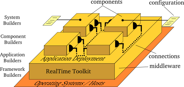
Figure 2.10, “ Component Deployment Levels ” shows the distinction between the three levels of Component Deployment.
Figure 2.10. Component Deployment Levels
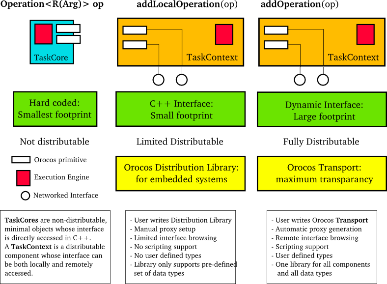
Three levels of using or creating Components can be accomplished in Orocos: Not distributed, embedded distributed and fully distributed.
If your application will not use distributed components and requires a very small footprint, the TaskCore can be used. The Orocos primitives appear publicly in the interface and are called upon in a hard-coded way.
If you application requires a small footprint and distributed components, the C++ Interface of the TaskContext can be used in combination with a Distribution Library which does the network translation. It handles a predefined set of data types (mostly the 'C' types) and needs to be adapted if other data types need to be supported. There is no portable distribution library available.
If footprint is of no concern to your application and you want to distribute any component completely transparently, the TaskContext can be used in combination with a Remoting Library which does the network translation. A CORBA implementation of such a library is being developed on. It is a write-once, use-many implementation, which can pick up user defined types, without requiring modifications. It uses the Orocos Type System to manage user defined types.
A TaskCore is nothing more than a place holder for the
Execution Engine and application code functions
(configureHook(), cleanupHook(),
startHook(), updateHook()
and stopHook() ). The Component
interface is built up by placing the Orocos primitives
as public class members in a TaskCore subclass. Each
component that wants to use this TaskCore must get a
'hard coded' pointer to it (or the interface it implements)
and invoke the command, method etc. Since Orocos is by
no means informed of the TaskCore's interface, it can not
distribute a TaskCore.
Instead of putting the Orocos primitives in the public interface of a subclass of TaskCore, one can subclass a TaskContext and register the primitives to the Local C++ Interface. This is a reduced interface of the TaskContext, which allows distribution by the use of a Distribution Library.
The process goes as such: A component inherits from TaskContext and has some Orocos primitives as class members. Instead of calling:
this->addOperation("name", &foo).doc("Description").arg("Arg1","Arg1 Description");and providing a description for the primitive as well as each argument, one writes:
this->addLocalOperation("name", &foo );This functions does no more than a pointer registration, but already allows all C++ code in the same process space to use the added primitive.
In order to access the interface of such a Component, the user code may use:
taskA->getLocalOperation("name");You can only distribute this component if an implementation of a Distribution Library is present. The specification of this library, and the application setup is in left to another design document.
In case you are building your components as instructed in this manual, your component is ready for distribution as-is, given a Remoting library is used. The Orocos CORBA package implements such a Remoting library.
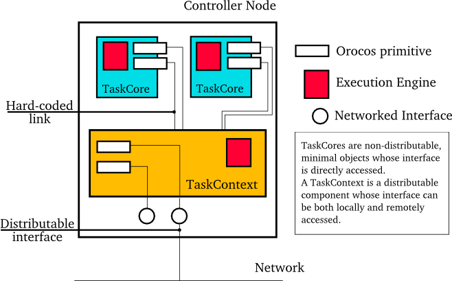
Using the three levels of deployment in one application is possible as well. To save space or execution efficiency, one can use TaskCores to implement local (hidden) functionality and export publicly visible interface using a TaskContext. Figure 2.11, “ Example Component Deployment. ” is an small example of a TaskContext which uses two TaskCores to delegate work to. The Execution Engines may run in one or multiple threads.
If you master the above methods of setting up tasks, this section gives some advanced uses for integrating your existing application framework in Orocos Tasks.
Most projects have define their own task interfaces in C++. Assume you have a class with the following interface :
  class DeviceInterface
  {
  public:
    /**
     * Set/Get a parameter. Returns false if parameter is read-only.
     */
    virtual bool setParameter(int parnr, double value) = 0;
    virtual double getParameter(int parnr) const = 0;

    /**
     * Get the newest data.
     * Return false on error.
     */
    virtual bool updateData() = 0;
    virtual bool updated() const = 0;

    /**
     * Get Errors if any.
     */
    virtual int getError() const = 0;
  };
Now suppose you want to do make this interface available, such that program scripts of other tasks can access this interface. Because you have many devices, you surely want all of them to be accessed transparently from a supervising task. Luckily for you, C++ polymorphism can be transparently adopted in Orocos TaskContexts. This is how it goes.
We construct a TaskContext, which exports your C++ interface to a task's interface.
  #include <rtt/TaskContext.hpp>
  #include <rtt/Operation.hpp>
  #include "DeviceInterface.hpp"

  class TaskDeviceInterface
    : public DeviceInterface,
      public TaskContext
  {
  public:
      TaskDeviceInterface()
        : TaskContext( "DeviceInterface" )
      {
         this->setup();
      }

      void setup()
      {
         // Add client thread operations :
         this->addOperation("setParameter",
                    &DeviceInterface::setParameter, this, ClientThread)
                        .doc("Set a device parameter.")
	                .arg("Parameter", "The number of the parameter.")
	                .arg("New Value", "The new value for the parameter.");

         this->addOperation("getParameter",
                     &DeviceInterface::getParameter, this, ClientThread)
                          .doc("Get a device parameter.")
                          .arg("Parameter", "The number of the parameter.");
         this->addOperation("getError",
                     &DeviceInterface::getError, this, ClientThread)
                          .doc("Get device error status.");

         // Add own thread operations :
         this->addOperation("updateData",
                          &DeviceInterface::updateData, this, OwnThread)
                              .doc(&DeviceInterface::updated)
                              .arg("Command data acquisition." );
      }
  };
The above listing just combines all operations which were introduced in the previous sections. Also note that the TaskContext's name is fixed to "DeviceInterface". This is not obligatory though.
Your DeviceInterface implementations now
only need to inherit from TaskDeviceInterface
to instantiate a Device TaskContext :
  #include "TaskDeviceInterface.hpp"

  class MyDevice_1
    : public TaskDeviceInterface
  {
  public:

    bool setParameter(int parnr, double value) {
      // ...
    }
    double getParameter(int parnr) const {      // ...
    }
    // etc.
  };
The new TaskContext can now be added to other tasks. If needed, an alias can be given such that the peer task knows this task under another name. This allows the user to access different incarnations of the same interface from a task.
	  // now add it to the supervising task :
  MyDevice_1 mydev;
  supervisor.addPeer( &mydev, "device" );
From now on, the "supervisor" task will be able to access "device". If the implementation changes, the same interface can be reused without changing the programs in the supervisor.
A big warning needs to be issued though : if you change a peer at run-time (after parsing programs), you need to reload all the programs, functions, state contexts which use that peer so that they reference the new peer and its C++ implementation.
To make the example complete, here is an example script which could run in the supervisor task :
  program ControlDevice
  {
     const int par1 = 0
     const int par2 = 1
     device.setParameter(par1, supervisor.par1 )
     device.setParameter(par2, supervisor.par2 )

     while ( device.getError() == 0 )
     {
        if ( this.updateDevice("device") == true )
           device.updateData()
     }
     this.handleError("device", device.getError() )
  }
To start this program from the TaskBrowser, browse to supervisor and type the command :
ControlDevice.start()
When the program "ControlDevice" is started, it initialises some parameters from its own attributes. Next, the program goes into a loop and sends updateData commands to the device as long as underlying supervisor (i.e. "this") logic requests an update and no error is reported. This code guarantees that no two updateData commands will intervene each other since the program waits for the commands completion or error. When the device returns an error, the supervisor can then handle the error of the device and restart the program if needed.
The advantages of this program over classical C/C++ functions are :
If any error occurs (i.e. a method returns false), the program stops and other programs or state contexts can detect this and take appropriate action.
The "
device.updateData()" call waits for completion of the remote operation.While the program waits for
updateData()to complete, it does not block other programs, etc within the same TaskContext and thread.There is no need for additional synchronisation primitives between the supervisor and the device since the operations have the OwnThread execution type. Which leads to :
The operation is executed at the priority of the device's thread, and not the supervisor's priority.
The operation can never corrupt data of the device's thread, since it is serialised(executed after) with the programs running in that thread.
Table of Contents
This document describes the Orocos Real-Time Scripting service
The Orocos Scripting language allows users of the Orocos system to write programs and state machines controlling the system in a user-friendly realtime script language. The advantage of scripting is that it is easily extendible and does not need recompilation of the main program.
Before starting to explain Program Syntax, it is necessary to explain some general concepts that are used throughout the program syntax.
Various sorts of comments are supported in the syntax. Here is a small listing showing the various syntaxes:
  # A perl-style comment, starting at a '#', and running until
  # the end of the line.

  // A C++/Java style comment, starting at '//', and running
  // until the end of the line.

  /* A C-style comment, starting at '/*', and running until
     the first closing */ /* Nesting is not allowed, that's
     why I have to start a new comment here :-)
  */
Whitespace is in general ignored, except for the fact that it is used to separate tokens.
Identifiers are names that the user can assign to variables, constants, aliases, labels. The same identifier can only be used once, except that for labels you can use an identifier that has already been used as a variable, constant or alias. However, this is generally a bad idea, and you shouldn't do it.
Some words cannot be used as identifiers, because they are reserved by the Orocos Scripting Framework, either for current use, or for future expansions. These are called keywords. The current list of reserved keywords is included here:
| alias | double | if | then |
| and | else | include | time |
| break | end | int | to |
| bool | export | next | true |
| char | local | not | try |
| catch | false | or | uint |
| const | for | return | until |
| define | foreach | set | var |
| do | global | string | while |
These, and all variations on the (upper- or lower-) case of each of the letters are reserved, and cannot be used as identifiers.
Expressions are a general concept used throughout the Parser system. Expressions represent values that can be calculated at runtime (like a+b). They can be used as arguments to functions, conditions and whatmore. Expressions implicitly are of a certain type, and the Parser system does strong type-checking. Expressions can be constructed in various ways, that are described below...
Literal values of various types are supported: string, int, double, bool. Boolean literals are either the word "true" or the word "false". Integer literals are normal, positive or negative integers. Double literals are C/C++ style double-precision floating point literals. The only difference is that in order for the Parser to be able to see the difference with integers, we require a dot to be present. String literals are surrounded by double quotes, and can contain all the normal C/C++ style escaped characters. Here are some examples:
  // a string with some escaped letters:
  "\"OROCOS rocks, \" my mother said..."
  // a normal integer
  -123
  // a double literal
  3.14159265358979
  // and another one..
  1.23e10
Constants, variables and aliases allow you to work with data in an easier way. A constant is a name which is assigned a value at parse time, and keeps that value throughout the rest of the program. A variable gets its value assigned at runtime and can be changed at other places in the program. An alias does not carry a value, it is defined with an expression, for which it acts as an alias or an abbreviation during the rest of the program. All of them can always be used as expressions. Here is some code showing how to use them.
  // define a variable of type int, called counter,
  // and give it the initial value 0.
  var int counter = 0
  // add 1 to the counter variable
  counter = counter + 1

  // make the name "counterPlusOne" an alias for the
  // expression counter + 1.  After this, using
  // counterPlusOne is completely equivalent to writing
  // counter + 1
  alias int counterPlusOne = counter + 1
  // you can assign an arbitrarily complex expression
  // to an alias
  alias int reallycomplexalias = ( ( counter + 8 ) / 3 )*robot.position

  // define a constant of type double, with name "pi"
  const double pi = 3.14159265358979
  const double pi2 = 2*pi       // ok, pi2 is 6.28...
  const int turn = counter * pi // warning ! turn will be 0 !

  // define a constant at _parse-time_ !
  const totalParams = table.getNbOfParams()
Variables, constants and aliases are defined for the following types: bool, int, double, string and array. The Orocos Typekit System allows any application or library to extend these types.
For convenience, two variable size types have been added to the parser : string and array. They are special because their contents have variable size. For example a string can be empty or contain 10 characters. The same holds for an array, which contains doubles. String and array are thus container types. They are mapped on std::string and std::vector<double>. To access them safely from a task method or command, you need to to pass them by const reference : const std::string& s, const std::vector<double>& v.
Container types can be used in two ways : with a predefined capacity (ie the possibility to hold N items), or with a free capacity, where capacity is expanded as there is need for it. The former way is necessary for real-time programs, the latter can only be used in non real-time tasks, since it may cause a memory allocation when capacity limits are exceeded. The following table lists all available constructors:
Table 3.1. array and string constructors
| Copy Syntax (copy done at run-time) | Pre-allocate syntax (init done at parse-time) | Notes |
|---|---|---|
var string x = string() | var string x | Creates an empty string. (std::string) |
var string x = string("Hello World") | var string x("Hello World") | Creates a string with contents "Hello World". |
var array x = array() | var array x | Creates an empty array. (std::vector<double>) |
var array x = array(10) | var array x(10) | Creates an array with 10 elements, all equal to 0.0. |
var array x = array(10, 3.0) | var array x(10, 3.0) | Creates an array with 10 elements, all equal to 3.0. |
var array x = array(1.0, 2.0, 3.0) | var array x(1.0, 2.0, 3.0) | Creates an array with 3 elements: {1.0, 2.0, 3.0}. Any number of arguments may be given. |
| Warning | |
|---|---|
The 'Copy Syntax' syntax leads to not real-time scripts because the size is expanded at run-time. See the examples below. |
Example 3.1. string and array creation
  // A free string and free array :
  // applestring is expanded to contain 6 characters (non real-time)
  var string applestring = "apples"

  // values is expanded to contain 15 elements (non real-time)
  var array  values      = array(15)

  // A fixed string and fixed array :
  var string fixstring(10)  // may contain a string of maximum 10 characters

  fixstring  = applestring   // ok, enough capacity
  fixstring  = "0123456789x" // allocates new memory (non real-time).


  var array  fixvalues(10)  // fixvalues pre-allocated 10 elements
  var array  morevalues(20) // arrays are initialised with n doubles of value 0.0

  fixvalues  = morevalues  // will cause allocation in 'fixvalues'
  morevalues = fixvalues   // ok, morevalues has enough capacity, now contains 10 doubles

  fixvalues  = morevalues  // ok, since morevalues only contains 10 items.

  values     = array(20)   // expand values to contain 20 doubles. (non real-time)

  var array list(1.0, 2.0, 3.0, 4.0) // list contains {1.0, 2.0, 3.0, 4.0}
  var array biglist;                 // creates an empty array
  biglist = list           // 'biglist' is now equal to 'list' (non real-time)
| Important | |
|---|---|
The 'size' value given upon construction (array(10) or string(17)) must be a legal expression at parse time and is only evaluated once. The safest method is using a literal integer ( i.e. (10) like in the examples ), but if you create a Task constant or variable which holds an integer, you can also use it as in : var array example( 5 * numberOfItems ) The expression may not contain any program variables, these will all be zero upon parse time ! The following example is a common mistake also : numberOfItems = 10 var array example( 5 * numberOfItems ) Which will not lead to '50', but to '5 times the value of numberOfItems, being still zero, when the program is parsed. |
Another property of container types is that you can index (use []) their contents. The index may be any expression that return an int.
  // ... continued
  // Set an item of a container :
  for (var int i=0; i < 20; i = i+1)
       values[i] = 1.0*i

  // Get an item of a container :
  var double sum
  for (var int i=0; i < 20; i = i+1)
       sum = sum + values[i]
If an assignment tries to set an item out of range, the assignment will fail, if you try to read an item out of range, the result will return 0.0, or for strings, the null character.
Expressions can be combined using the C-style operators that you are already familiar with if you have ever programmed in C, C++ or Java. Most operators are supported, except for the if-then-else operator ("a?b:c") and the "++/--" post-/pre- increment operators. The precedence is the same as the one used in C, C++, Java and similar languages. In general all that you would expect, is present.
When a data type is a C++ struct or class, it contains fields which you might want to access directly. These can be accessed for reading or writing by using a dot '.' and the name of the field:
  var mydata d1;

  d1.count = 1;
  d1.name  = "sample";
Some value types, like array and string, are containing read-only values or useful information about their size and capacity:
  var string s1 = "abcdef"

  // retrieve size and capacity of a string :
  var int size = s1.size
  var int cap  = s1.capacity
  var array a1( 10 )
  var array a2(20) = a1

  // retrieve size and capacity of a array :
  var int size = a2.size      // 10
  var int cap  = a2.capacity  // 20
Before we go on describing the details of the programs syntax, we show how you can load a program in your Real-Time Task.
The easiest way is to use the DeploymentComponent where you can specify a script to load in the application's deployment XML file or using the TaskBrowser. You can also do it in C++, as described below.
The example below is for a program script
programs.ops which contains a program
with the name "progname".
This is the easiest procedure. You need to tell the taskbrowser that you want the scripting service and then use the scripting service to load the program script:
  Component [R]> .provide scripting
  Trying to locate service 'scripting'...
  Service 'scripting' loaded in Component
  Component [R]> scripting.loadPrograms("programs.ops")
    = true
  Component [R]> progname.start()
    = true
Parsing the program is done using the 'getProvider' function to call the scripting service's functions:
  #include <rtt/Activity.hpp>
  #include <rtt/TaskContext.hpp>
  #include <rtt/scripting/Scripting.hpp>

  using namespace RTT;

  TaskContext   tc;
  tc.setActivity( new Activity(5, 0.01) );

  // Watch Logger output for errors :
  tc.getProvider<Scripting>("scripting")->loadPrograms("program.ops");

  // start a program :
  tc.getProvider<Scripting>("scripting")->startProgram("progname");
The Scripting service will load all programs and functions into 'tc'.The program "progname" is then started. Programs can also be started from within other scripts.
In case you wish to have a pointer to a program script object (ProgramInterface), you can have so only from within the owner TaskContext by writing:
  // Services are always accessed using a shared_ptr
  // cast the "scripting" RTT::Service to an RTT::scripting::ScriptingService shared_ptr:
  RTT::scripting::ScriptingService::shared_ptr ss
     = boost::dynamic_pointer_cast<ScriptingService>( this->provides()->getService("scripting") );

  ProgramInterfacePtr p = ss->getProgram("progname");

  // start a program :
p->start();An Orocos program script is a list of statements, quite similar to a C program. Programs can call C/C++ functions and functions can be loaded into the system, such that other programs can call them. Program scripts are executed by the Execution Engine.
In general, program statements are executed immediately one after the other. However, when the program needs to wait for a result, the Execution Engine temporarily postpones program execution and will try again in the next execution period. This happens typically when yield was called. Calling operations and expressions on the other hand typically do not impose a yield, and thus are executed immediately after each other.
A program is formed like this:
  program progname {
    // an arbitrary number of statements
  }
The statements are executed in order, starting at the first and following the logical execution path imposed by your program's structure. If any of the statements causes a run-time error, the Program Processor will put the program in the error state and stop executing it. It is the task of other logic (like state machines, see below) to detect such failures.
A variable is declared with the var keyword and can be changed using the = symbol. It looks like this:
  var int a, b, c;
  a = 3 * (b = (5 * (c = 1))); // a = 15, b = 5, c = 1
The semicolon at the end of the line is optional, but when omitted, a newline must be used to indicate a new statement.
A Program script can contain if..then..else blocks, very similar to C syntax, except that the then word is mandatory and that the braces () can be omitted. For example:
  var int x = 3

  if x == 3 then  x = 4
  else x = 5

  // or :
  if (x == 3) then {
    x = 4
    // ...
  } else {
    x = 5
    // ...
  }
It is thus possible to group statements. Each statement can be another if clause. An else is always referring to the last if, just like in C/C++. If you like, you can also write parentheses around the condition. The else statement is optional.
The for statement is almost equal to the C language. The first statement initialises a variable or is empty. The condition contains a boolean expression (use 'true' to simulate an empty condition). The second statement changes a variable or is empty.
  // note the var when declaring i:
  for ( var int i = 0; i != 10; i = i + 1 )
        log("Hello World")
  // or group:
  for ( i = 0; i < b; i = i + 1 ) {
        log("In the loop")
        // ...
  }
Note that Orocos scripting does not (yet) support the postfix or prefix increment/decrement operators like ++ and --.
The while statement is another looping primitive in the Orocos script language. A do statement is not implemented
  var int i = 0;
  while i < 10
      i = i +1
  // or group:
  i = 0;
  while i < 10 {
      log("In while")
      i = i + 1
      // ...
  }
As with the if statement, you can optionally put parentheses around the condition 'i < 10'. Note that Orocos scripting does not support the postfix or prefix increment/decrement operators like ++ and --.
To break out of a while or for loop, the break statement is available. It will break out of the innermost loop, in case of nesting.
  var int i = 0
  while true  {
      i = i + 1
      if i == 50 then
          break
      // ...
  }
It can be used likewise in a for loop.
Operations can be called like calling C functions. They take arguments and return a value immediately. They can be used in expressions or stand alone :
  // var int arg1 = 3, arg2 = 4
  // ignore the return value :
  peer.method( arg1, arg2 )

  // this will only work if the method returns a boolean :
  if ( peer.method( arg1, arg2 ) ) {
  	    // ...
  }

  // use another method in an expression :
  data = comp.getResult( arg1 ) * 20. / comp.value
These operations are executed directly one after the other.
| Warning | |
|---|---|
A method throwing an exception, will cause a run-time program error. If this is not wanted, put 'try' in front of the method call statement, as shown in the next section. |
When a method throws a C++ exception, the program goes into an error state and waits for user intervention. This can be intercepted by using a try...catch statement. It tries to execute the method, and if it throws, the optional catch clause is executed :
  // just try ignores the exception of action :
  try comp.action( args )

  // When an exception is thrown, execute the catch clause :
  try comp.action( args ) catch {
      // statements...
  }
If the method did not throw, the catch clause is not executed. Note that you can not inspect the C++ exception, so only rudimentary error handling is available.
Task attributes/Properties are set in the same way as ordinary script variables.
  // Setting a property named MyProp of type double
  var double d = 5.0
  comp.MyProp = d
Statements can be grouped in functions. A function can only call another function which is earlier defined. Thus recursive function calling is not allowed in this language.
  // A function only known in the current scripting service
  void func_name( int arg1, double arg2 ) {
    // an arbitrary number of statements
  }

  // A function put in the interface of the component
  export double func_name(bool arg) {
    // ...
    if ( arg ) then return +10.0; else return -10.0;
  }

  // A function put in the global service interface of the current process
  global double global_func_name(bool arg) {
    // ...
    if ( arg ) then return +10.0; else return -10.0;
  }
A function can have any number of arguments, which are passed by value, and may return a value.
By default, a function is only known in the scripting service of the current component. You can make this explicit by writing the local keyword in front of the return value. This function will be found as an operation in the 'scripting' Service of the current component. You should not rely on the presence or name of this Operation, since it is considered as 'internal' to the scripting Service. Future releases may relocate or rename this function.
You can add a function to the interface of the current component by using the export keyword. This allows you to extend the interface of a component at run-time.
Finally, the global keyword puts the defined function in the GlobalService, which makes it available for any component or script in the current process.
You may redefine a function with the same name, in which case a warning will be logged and the new function is installed. In case the same function name is in use locally, at the TaskContext interface or globally, the local function is used first, then the TaskContext function and finally the global function.
A function can be called as a regular Operation :
foo(arg) // is a global, local or exported function of the current component
If one of the statements of the called function throws an exception, an exception is thrown in the current program and the calling program goes into the error state.
| Note | |
|---|---|
The 'call' keyword has been deprecated since version 2.5 and should no longer be used. |
The return statement behaves like in traditional languages. For programs and functions that do not return a value, the return statement is written like:
  export void foo(int i) {
     // ...
     if ( i < 0 )
        return
     // use i...
  }
When the return statement returns a value, it must be on the same line as the return word:
  export int foo(int i) {
     // ...
     if ( i < 0 )
        return -1  // returned value on same line.
     // use i...
     return i*10
  }
As the examples show, you can return from a function from multiple places.
A special statement 'yield' is provided. It temporarily suspends the execution of the current script and allows the Execution Engine in which it runs to do something else. You will need this in an endless while loop, for example:
  while( true ) {
    log("Waiting...")
    yield
  }
If the yield statement is omitted, the script would never return and consume all available processor time. Yield suspends the execution of this script until the ExecutionEngine is triggered again, for example, when an asynchronous operation is received or by the expiration of the period in a periodically running component.
Once a program is parsed and loaded into the Execution Engine, it can be manipulated from another script. This can be done through the programs subtask of the TaskContext in which the program was loaded. Assume that you loaded "progname" in task "ATask", you can write
  ATask.progname.start()
  ATask.progname.pause()
  ATask.progname.step()
  ATask.progname.step()
  ATask.progname.stop()
The first line starts a program. The second line pauses it. The next two lines executes one command each of the program (like stepping in a debugger). The last line stops the program fully (running or paused).
Some basic properties of the program can be inspected likewise :
  var bool res =  ATask.progname.isRunning()
  res = ATask.progname.inError()
  res = ATask.progname.isPaused()
which all return a boolean indicating true or false.
A StateMachine is the state machine used in the Orocos system. It contains a collection of states, and each state defines a Program on entry of the state, when it is run and on exit. It also defines all transitions to a next state. Like program scripts, a StateMachine must be loaded in a Task's Execution Engine.
A StateMachine is composed of a set of states. A running StateMachine is always in exactly one of its states. One time per period, it checks whether it can transition from that state to another state, and if so makes that transition. By default, only one transition can be made in one Execution Engine step.
Besides a list of the possible transitions, every state also keeps record of programs to be executed at certain occasions. There can be up to four (all optional) programs in every state: the entry program ( which will be executed each time the state is entered ), the run program ( which will be executed every time the state is the active state ), the handle program ( which will be executed right after run, if no transition succeeds ) and the exit program ( which will be executed when the state is left).
There can be more than one StateMachine. They separately keep track of their own current state, etc.
A StateMachine can have any number of states. It needs to have exactly one "initial state", which is the state that will be entered when the StateMachine is first activated. There is also exactly one final state, which is automatically entered when the StateMachine is stopped. This means that the transition from any state to the final state must always be meaningful.
A State Machine can run in two modes. They are the automatic mode and the reactive (also 'event' or 'request') mode. You can switch from one mode to another at run-time.
In order to enter the reactive mode, the State Machine must be 'activated'. When active, two possible causes of state transitions can exist: because an event occured or because a transition was requested.
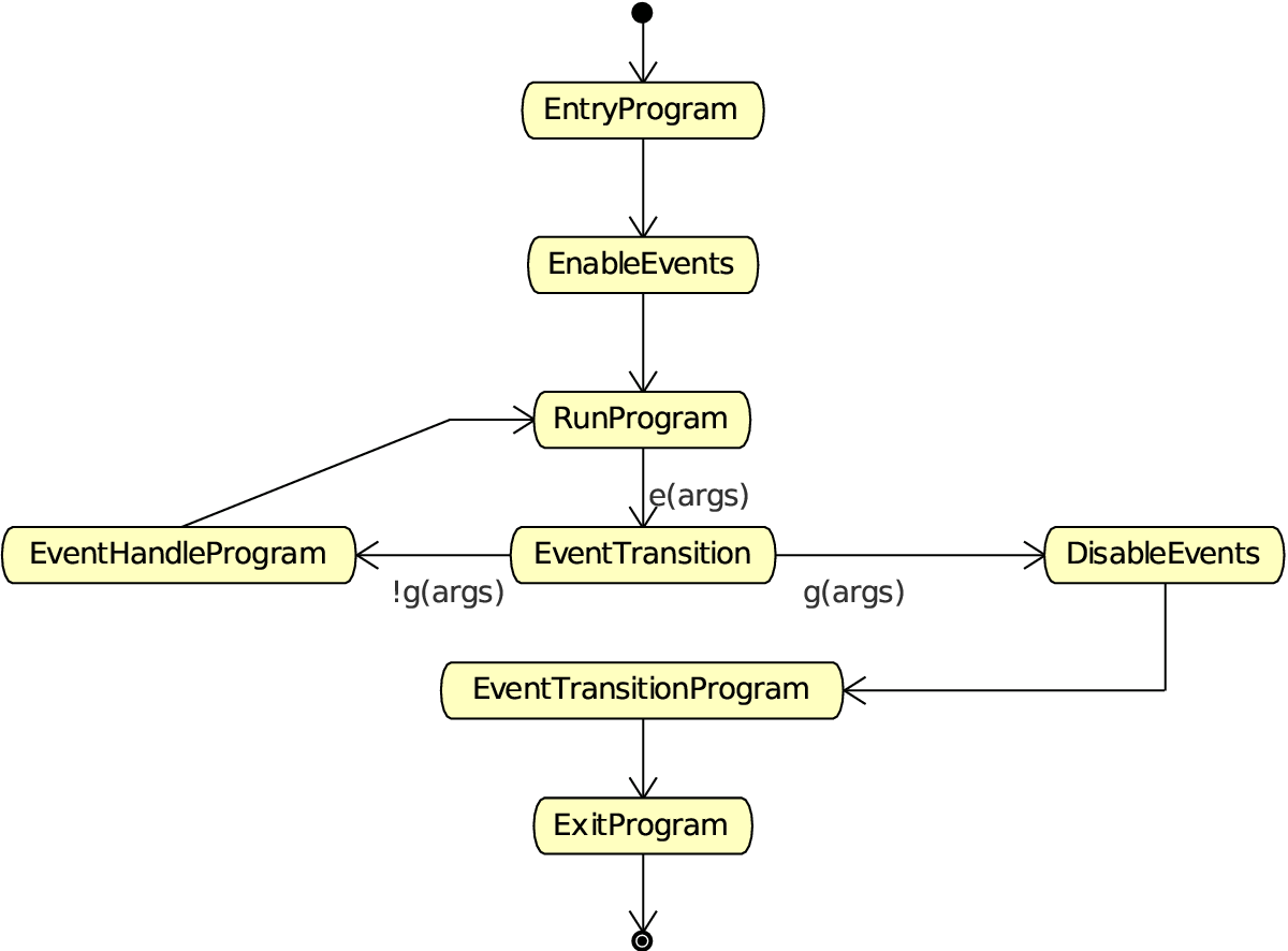
A state can list to which Orocos data flow events it reacts, and under which conditions it will make a transition to another state. A state only reacts to events when its entry program is fully executed (done) and an event may be processed when the run program is executed, thus interrupt the run program. The first event that triggers a transition will 'win' and the state reacts to no more events, executes the event's transition program, then the state's exit program, and finally, the next state is entered and its entry program is executed. The next state now listens for events (if any) to make a transition or just executes its run program.
Another program can request a transition to a particular state as well. When the request arrives, the current state checks its transition conditions and evaluates if a transition to that state is allowed. These conditions are separately listed from the event transitions above. If a transition condition is valid, the exit program of the current state is called, the transition program and then the entry program of the requested state is called and the requested state's run program is executed. If a transition to the current state was requested, only the run program of the current state is executed.
In this mode, it is also possible to request a single transition to the 'best' next state. All transition conditions are evaluated and the first one that succeeds makes a transition to the target state. This mechanism is similar to automatic mode below, but only one transition is made ( or if none, handle is executed ) and then, the state machine waits again. The step() command triggers this behaviour.
In order to enter automatic mode, the State Machine must be first reactive and then started with the start() command (see later on).
| Note | |
|---|---|
This mechanism is in addition to 'reactive' mode. A state machine in automatic mode still reacts to events. |
Figure 3.2. State Change Semantics in Automatic Mode
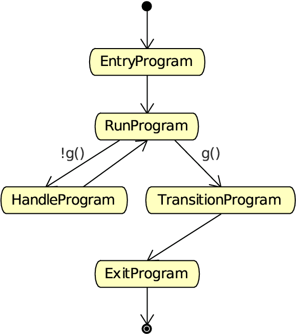 |
The automatic mode additionally actively evaluates guard conditions. Event reaction remains in effect, but is not shown in this diagram.
In automatic mode, after the run program of the current state finishes, the transition table (to other states) of the current state is evaluated. If a transition succeeds, the transition program is executed, then the exit program of the current state is called and then the entry program of the next state is called. If no transition evaluated to true, the handle program (if any) of the current state is called. This goes on until the automatic mode is left, using the pause, stop or reactive command.
Analogous to the Program section, we first show how
you can load a StateMachine in your Real-Time Task.
Assume that you have a StateMachine "MachineInstanceName"
in a file state-machine.osd.
This is the easiest procedure. You need to tell the taskbrowser that you want the scripting service and then use the scripting service to load the state machine
  Component [R]> .provide scripting
  Trying to locate service 'scripting'...
  Service 'scripting' loaded in Component
  Component [R]> scripting.loadStateMachines("state-machine.osd")
    = true
  Component [R]> MachineInstanceName.activate()
    = true
  Component [R]> MachineInstanceName.start()
    = true
Parsing the StateMachine is very analogous to parsing Programs in C++:
  #include <rtt/Activity.hpp>
  #include <rtt/TaskContext.hpp>
  #include <rtt/scripting/Scripting.hpp>

  using namespace RTT;

  TaskContext   tc;
  tc.setActivity( new Activity(5, 0.01) );

  tc.getProvider<Scripting>("scripting")->loadStateMachines( "state-machine.osd" );

  // activate a state machine :
  tc.getProvider<Scripting>("scripting")->activateStateMachine("MachineInstanceName");
  // start a state machine (automatic mode) :
  tc.getProvider<Scripting>("scripting")->startStateMachine("MachineInstanceName");
The Scripting service loads all instantiated state machines in tc. StateMachines have a more complex lifetime than Programs. They need first to be activated, upon which they enter a fixed initial state. When they are started, they enter automatic mode and state transitions to other states can take place. StateMachines can also be manipulated from within other scripts.
In case you wish to have a pointer to a state machine script object (StateMachine), you can have so only from within the owner TaskContext by writing:
  // Services are always accessed using a shared_ptr
  // cast the "scripting" RTT::Service to an RTT::scripting::ScriptingService shared_ptr:
  RTT::scripting::ScriptingService::shared_ptr ss
     = boost::dynamic_pointer_cast<ScriptingService>( this->provides()->getService("scripting") );

  StateMachinePtr sm = ss->getStateMachine("MachineInstanceName");

  // activate and start a StateMachine :
  sm->activate();
sm->start();You can think of StateMachines somewhat like C++ classes. You first need to define a type of StateMachine, and you can then instantiate it any number of times afterwards. A StateMachine ( the type ) can have parameters, so every instantiation can work differently based on the parameters it got in its instantiation.
A StateMachine definition looks like this :
Example 3.2. StateMachine Definition Format
  StateMachine MyStateMachineDefinition
  {
    initial state myInit
    {
        // all these programs are optional and can be left out:
        entry {
	    // entry program
	}
	run {
	    // run program
	}
	handle {
	    // handle program
	}
	exit {
	    // exit program
	}
	// Ordered event based and conditional select statements
	transition ... { /* transition program */ } select ...
	transition ...

    }

    final state myExit {
	entry {
	    // put everything in a safe state.
	}
	// leave out empty programs...

	transition ...
    }

    state Waiting {
        // ...
    }

    // ... repeat
  }

  // See Section 5.5, “Instantiating Machines: SubMachines and RootMachines” :
  RootMachine MyStateMachineDefinition MachineInstanceName
A StateMachine definition: a StateMachine can have any number of states. It needs to have exactly one "initial state" ( which is the state that will be entered when the StateMachine is first started ). Within a state, any method is optional, and a state can even be defined empty.
A state machine can have an unlimited number of states. A state contains optionally 4 programs : entry, run, handle, exit. Any one of them is optional, and a state can even conceivably be defined empty.
When a state is entered for the first time, the entry program is executed. When it is left, the exit program is called. The execution semantics are identical to the program scripts above.
The run program serves to define which activity is done within the state. After the entry program finishes, the run program is immediately started. It may be interrupted by the events that state reacts to. In event mode, the run program is executed once (although it may use an infinite loop to repeatedly execute statements). In automatic mode, when the run program completes, and no transitions to another state can be made (see below) it is started again (in the next execution step).
When the run program finishes in automatic mode, the
state evaluates its transitions to other states.
The handle program is called only when no transition can be found to another state.
The transitions section defines one or more select
state statements. These can be guarded by if...then clauses
(the transition conditions):
  // In state XYZ :
  // conditionally select the START state
  transition if HMI.startPushed then {
        // (optional)
        // transition program: HMI.startPushed was true
        // when finished, go to START state
  } select START

  // next transition condition, with a transition failure program:
  transition if HMI.waiting then
      select WAIT else {
        // (optional)
        // transition failure program: HMI.startPushed was false
  }

  handle {
     // only executed if no transition above could be made
     // if startPushed and waiting were false:
     // ...
  }
The transitions are checked in the same order as listed. A transition is allowed to select the current state, but the exit and entry functions will not be called in that case. Even more, a transition to the current state is always considered valid and this can not be overridden.
Often it's useful to specify some preconditions that need to hold before entering a state. Orocos states explicitly allow for this. A state's preconditions will be checked before the state is entered.
Preconditions are specified as follows:
  state X {
    // make sure the robot is not moving axis 1 when entering this state
    // and a program is loaded.
    precondition  robot.movingAxis( 1 ) == false
    precondition  programLoaded == true
    // ...
  }
They are checked in addition to transitions to that state and can make such a transition fail, hence block the transition, as if the transition condition in the first place did not succeed.
An important property of state machines is that they can react to external (asynchronous) events. Orocos components can define reactions to data arriving on InputPorts. When new data arrives on this port, we speak of an 'event'.
| Note | |
|---|---|
A StateMachine can only react to InputPorts which have been added with 'addEventPort' to the TaskContext. |
Event transitions are an extension to the transitions above and cite an InputPort name between the transition and the if statement. They are specified as:
  state X {
    var double d
    transition x_in_port(d) if ( d >1.3 ) then {
       // transition succeeds, transition program:
       // ...
    } select ONE_STATE else {
       // transition fails, failure program:
       // ...
    } select OTHER_STATE

    // other events likewise...
  }
Both the transition programs and the the select statements are optional, but at least a program or select statement must be given. The
transition x_in_port(d) if (d >1.3) then {
short notation statement is equivalent to writing:
transition if ( x_in_port(d) == NewData && d >1.3) then {...
| Important | |
|---|---|
This short notation differs however from the long form as such: if multiple transitions are waiting on the same port, but with a different guard, the short notation will give all transitions a chance to see the NewData return value. If a user would use the long form, only the first transition statement would see NewData, all the others would see OldData as return value. Hence the short notation is prefered. |
When the input port x_in_port
receives NewData, our state machine reacts to it and the
data is stored in d. The if ... then
statement may check this variable and any other state
variables and methods to evaluate the transition. If it
succeeds, an optional transition program may be given and
a target state selected (ONE_STATE).
if the transition fails, an optional failure program may
be given and an optional select
(OTHER_STATE) statement may be given. The number of
arguments must match the number of arguments of the used
event. The event is processed as an asynchronous
callback, thus in the thread or task of the StateMachine's
processor.
Event transitions are enabled after the entry program and before the exit program (also in automatic mode). All events are processed in a state until the first event that leads to a valid state transition. In the mean time, the run program or handle programs may continue, but will be interrupted if an event occurs. The event transition program and/or exit program may or must thus perform the necessary cleanup.
As mentioned before: you can look at a SubMachine definition as the definition of a C++ class. It is merely the template for its instantiations, and you have to instantiate it to actually be able to do anything with it. There is also a mechanism for passing parameter values to the StateMachines on instantiation.
Note that you always need to write the instantiation after the definition of the StateMachine you're instantiating.
A Root Machine is a normal instantiation of a StateMachine, one that does not depend on a parent StateMachine ( see below ). They are defined as follows:
  StateMachine SomeStateMachine
  {
      initial state initState
      {
        // ...
      }
      final state finalState
      {
        // ...
      }
  }

  RootMachine SomeStateMachine someSMinstance
This makes an instantiation of the StateMachine type SomeStateMachine by the name of 'someSMinstance', which can then be accessed from other scripts (by that name).
You can define variables at the StateMachine level. These variables are then accessible to the StateMachine methods (entry, handle, exit), the preconditions, the transitions and ( in the case of a SubMachine, see below ) the parent Machine.
You can define a StateMachine public variable as follows:
  StateMachine SomeStateMachine
  {
    // a public constant
    const double pi = 3.1415926535897
    var int counter = 0

    initial state initState
    {
	handle
	{
            // change the value of counter...
            counter = counter + 1
        }
        // ...
    }
    final state finalState
    {
	entry
        {
            someTask.doSomethingWithThisCounter( counter )
        }
        // ...
    }
  }

  Rootmachine SomeStateMachine mymachine
This example creates some handy public variables in the StateMachine SomeStateMachine, and uses them throughout the state machine. They can also be read and modified from other tasks or programs :
  var int readcounter = 0
  readcounter = taskname.mymachine.counter

  taskname.mymachine.counter = taskname.mymachine.counter *  2
A StateMachine can have parameters that need to be set on its instantiation. Here's an example:
  StateMachine AxisController
  {
      // a parameter specifying which axis this Controller controls
      param int axisNumber
      initial state init
      {
          entry
          {
              var double power = someTask.getPowerForAxis( axisNumber )
  	    // do something with it...
          }
      }
  }

  RootMachine AxisController axiscontroller1( axisNumber = 1 )
  RootMachine AxisController axiscontroller2( axisNumber = 2 )
  RootMachine AxisController axiscontroller3( axisNumber = 3 )
  RootMachine AxisController axiscontroller4( axisNumber = 4 )
  RootMachine AxisController axiscontroller5( axisNumber = 5 )
  RootMachine AxisController axiscontroller6( axisNumber = 6 )
This example creates an AxisController StateMachine with one integer parameter called axisNumber. When the StateMachine is instantiated, values for all of the parameters need to be given in the form "oneParamName= 'some value', anotherParamName = 0, yetAnotherParamName=some_other_expression + 5". Values need to be provided for all the parameters of the StateMachine. As you see, a StateMachine can of course be instantiated multiple times with different parameter values.
A SubMachine is a StateMachine that is instantiated within another StateMachine ( which we'll call the parent StateMachine ). The parent StateMachine is owner of its child, and can decide when it needs to be started and stopped, by invoking the respective methods on its child.
An instantiation of a SubMachine is written as follows:
  StateMachine ChildStateMachine
  {
      initial state initState
      {
          // ...
      }
      final state finalState
      {
          // ...
      }
  }

  StateMachine ParentStateMachine
  {
      SubMachine ChildStateMachine child1
      SubMachine ChildStateMachine child2
      initial state initState
      {
  	entry
          {
	      // enter initial state :
  	    child1.activate()
  	    child2.activate()
          }
          exit
          {
	      // enter final state :
              child2.stop()
          }
      }

      final state finalState
      {
          entry
          {
	      // enter final state :
              child1.stop()
          }
      }
  }
Here you see a ParentStateMachine which has two ChildStateMachines. One of them is started in the initial state's entry method and stopped in its exit method. The other one is started in the initial state's entry method and stopped in the final state's entry method.
In addition to starting and stopping a SubMachine, a parent StateMachine can also inspect its public variables, change its parameters, and check what state it is in...
Inspecting StateMachine public variables is simply done using the syntax "someSubMachineInstName.someValue", just as you would do if someSubMachineInstName were an Orocos task. Like this, you can inspect all of a subcontext's public variables.
Setting a StateMachine parameter must be done at its instantiation. However, you can still change the values of the parameters afterwards. The syntax is: "set someSubMachine.someParam = someExpression". Here's an elaborate example:
  StateMachine ChildStateMachine
  {
      param int someValue
      const double pi = 3.1415926535897
      initial state initState
      {
          // ...
      }
      final state finalState
      {
          // ...
      }
  }

  StateMachine ParentStateMachine
  {
      SubMachine ChildStateMachine child1( someValue = 0 )
      SubMachine ChildStateMachine child2( someValue = 0 )

      var int counter = 0
      initial state initState
      {
  	  entry
          {
  	      child1.start()
  	      child2.start()
              // set the subcontext's parameter
              child1.someValue = 2
          }
          run
          {
              counter = counter + 1
              // set the subcontext's parameters
              child2.someValue = counter
              // use the subcontext's public variables
              someTask.doSomethingCool( child1.someValue )
          }
          exit
          {
              child2.stop()
          }
      }

      final state finalState
      {
          entry
          {
              child1.stop()
          }
      }
  }
You can also query if a child State Machine is in a certain state. The syntax looks like:
someSubMachine.inState( "someStateName" )
Once a state machine is parsed and loaded into the State Machine Processor, it can be manipulated from another script. This can be done through the "states" subtask of the TaskContext in which the state machine was loaded. Assume that you loaded "machine" with subcontexts "axisx" and "axisy" in task "ATask", you can write
  ATask.machine.activate()
  ATask.machine.axisx.activate()
  // now in reactive mode...

  ATask.machine.axisx.start()
  ATask.machine.start()
  // now in automatic mode...

  ATask.machine.stop()
  // again in reactive mode, in final state

  ATask.machine.reset()
  ATask.machine.deactivate()
  // deactivated.
  // etc.
The first line activates a root StateMachine, thus it enters the initial state and is put in reactive mode , the next line actives its child, the next starts its child, then we start the parent, which bring both in automatic mode. Then the parent is stopped again, reset back to its initial state and finally deactivated.
Thus both RootMachines and SubMachines can be controlled. Some basic properties of the states can be inspected likewise :
  var bool res =  ATask.machine.isActive()      // Active ?
  res = ATask.machine.axisy.isRunning()     // Running ?
  res =  ATask.machine.isReactive()          // Waiting for requests or events?
  var string current = ATask.machine.getState() // Get current state
  res = ATask.machine.inState( current )    // inState ?
which makes it possible to monitor state machines from other scripts or an operator console.
Consider the following StateMachine :
  StateMachine X {
     // ...
     initial state y {
        entry {
	   // ...
        }
       // guard this transition.
       transition if checkSomeCondition() then
              select z
       transition if checkOtherCondition() then
              select exit
     }
     state z {
       // ...
       // always good to go to state :
       transition select ok_1
	  select ok_1
     }
     state ok_1 {
       // ...
     }
     final state exit {
       // ...
     }
  }

  RootMachine X x
A program interacting with this StateMachine can look like this :
   program interact {
       // First activate x :
       x.activate()  // activate and wait.

       // Request a state transition :
       try x.requestState("z") catch {
           // failed !
       }

       // ok we are in "z" now, try to make a valid transition :
       x.step()

       // enter pause mode :
       x.pause()
       // Different ! Executes a single program statement :
       x.step()

       // unpause, by re-entering reactive Mode :
       x.reactive()

       // we are in ok_1 now, again waiting...
       x.stop()      // go to the final state

       // we are in "exit" now
       reset()

       // back in state "y", handle current state :
       this.x.requestState( this.x.getState() )
       // etc.
    }
The requestState command will fail if the transition is not possible ( for example, the state machine is not in state y, or checkSomeCondition() was not true ), otherwise, the state machine will make the transition and the command succeeds and completes when the z state is fully entered (it's init program completed).
The next command, step(), lets the state machine decide which state to enter, and since a transition to state "ok_1" is unconditionally, the "ok_1" state is entered. The stop() command brings the State Machine to the final state ("exit"), while the reset command sends it to the initial state ("y"). These transitions do not need to be specified explicitly, they are always available.
The last command, is a bit cumbersome request to execute the handle program of the current state.
At any time, the State Machine can be paused using pause(). The step() command changes to execute a single program statement or transition evaluation, instead of a full state transition.
All these methods can of course also be called from parent to child State Machine, or across tasks.
Consider the following StateMachine, as in the previous section :
  StateMachine X {
     // ...
     initial state y {
        entry {
	   // ...
        }
        // guard this transition.
        transition if checkSomeCondition() then
              select z
        transition if checkOtherCondition() then
              select exit
     }
     state z {
       // ...
       // always good to go to state :
       transition select ok_1
     }
     state ok_1 {
       // ...
     }
     final state exit {
       // ...
     }
  }

  RootMachine X x
A program interacting with this StateMachine can look like this :
   program interact {
       // First activate x :
       x.activate()  // activate and wait.

       // Enter automatic mode :
       x.start()

       // pause program execution :
       x.pause()

       // execute a single statement :
       x.step()

       // resume automatic mode again :
       x.start()

       // stop, enter final state, in request mode again.
       x.stop()

       // etc...
    }
After the State Machine is activated, it is started, which lets the State Machine enter automatic mode. If checkSomeCondition() evaluates to true, the State Machine will make the transition to state "z" without user intervention, if checkOtherCondition() evaluates to true, the "exit" state will be entered.
When running, the State Machine can be paused at any time using pause(), and a single program statement ( a single line ) or single transition evaluation can be executed with calling step(). Automatic mode can be resumed by calling start() again.
To enter the reactive mode when the State Machine is in automatic mode, one can call the reactive() command, which will finish the program or transition the State Machine is making and will complete if the State Machine is ready for requests.
All these methods can of course also be called from parent to child State Machine, or across tasks.
This sections shows the listings of an Orocos State Description and an Orocos Program Script. They are fictitious examples (but with valid syntax) which may differ from actual available tasks. The example tries to exploit most common functions.
Example 3.3. StateMachine Example (state.osd)
The Example below shows a state machine for controlling 6 axes.
    StateMachine Simple_nAxes_Test
    {

      var bool calibrate_offsets     = true
      var bool move_to               = true
      var bool stop                  = true

      const double pi = 3.14159265358979
      var array pos = array(6,0.0)


      initial state StartRobotState {
        entry {
          Robot.prepareForUse()
        }
        exit {
          Robot.unlockAllAxes()
          Robot.startAllAxes()
        }
        transitions {
          select CalibrateOffsetsState
        }
      }


      state CalibrateOffsetsState {
        preconditions {
          if (calibrate_offsets == false) then
            select MoveToState
        }
        entry {
          nAxesGeneratorPos.start()
          nAxesControllerPos.start()
          //Reporter.start()
          CalibrateOffsetsProg.start()
        }
        exit {
          nAxesGeneratorPos.stop()
          nAxesControllerPos.stop()
        }
        transitions {
           if !CalibrateOffsetsProg.isRunning then
           select MoveToState
        }
      }


      state MoveToState {
        preconditions {
          if (move_to == false) then
            select StopRobotState
        }
        entry {
          nAxesGeneratorPos.start()
          nAxesControllerPosVel.start()
          pos = array(6,0.0)
          nAxesGeneratorPos.moveTo(pos,0.0)
          pos[0]=-pi/2.0
          pos[1]=-pi/2.0
          pos[2]=pi/2.0
          pos[4]=-pi/2.0
          nAxesGeneratorPos.moveTo(pos,0.0)
        }
        exit {
           nAxesControllerPosVel.stop()
           nAxesGeneratorPos.stop()
           //Reporter.stop()
        }
        transitions {
          if(stop == true) then
          select StopRobotState
        }
      }


      final state StopRobotState {
        entry {
          Robot.stopAllAxes()
          Robot.lockAllAxes()
        }
        exit {
          Robot.prepareForShutdown()
        }
      }
    }
    RootMachine Simple_nAxes_Test SimpleMoveTo
  /**
   * This program is executed in the exec_state.
   */

  /**
   * Request the HMI to load the user selected
   * trajectory into the kernel.
   */
  export function HMILoadTrajectory() {
  	// request a 'push' of the next
  	// trajectory :
  	HMI.requestTrajectory()
  	// when the HMI is done :
  	Generator.loadTrajectory()
  }

  /**
   * a Homing (reset) of the axes.
   * This could also be done using a Homing state,
   * without a program.
   */
  export function ResetAxes() {
  	HomingGenerator.start()
  	HomingGenerator.homeAll()
  }

  export function ResetAxis(int nr) {
  	HomingGenerator.start()
  	HomingGenerator.homeAxis( nr )
  }

  /**
   * Request the Generator to use the current
   * trajectory.
   */
  function runTrajectory() {
  	Generator.startTrajectory()
  	// this function returns when the
  	// trajectory is done.
  }

  program DemoRun {
  	HMI.display("Program Started\n")
  	var int cycle = 0

  	// We actually wait here until a
  	// Trajectory is present in the HMI.
  	while ( !HMI.trajectoryPresent() )
	   yield;

  	while HMI.cycle() {
  	    HMI.display("Cycle nr: %d.\n", cycle )
  	    ResetAxes()
  	    HMIRequestTrajectory()
  	    runTrajectory()

  	    Timer.sleep( 5.0 ) // wait 5s
  	}

  	HMI.display("Program Ended\n")
} Table of Contents
This document explains the principles of the Corba Transport of Orocos, the Open RObot COntrol Software project. It enables transparant deployment accross networked nodes of plain Orocos C++ components.
This transport allows Orocos components to live in separate processes, distributed over a network and still communicate with each other. The underlying middleware is CORBA, but no CORBA knowledge is required to distribute Orocos components.
The Corba transport provides:
Connection and communication of Orocos components over a network or between two processes on the same computer.
Clients (like visualisation) making a connection to any running Orocos component using the IDL interface.
Transparant use: no recompilation of existing components required. The library acts as a run-time plugin.
| Important | |
|---|---|
Follow these instructions carefully or your setup will not work ! |
In order to distribute Orocos components over a network, your computers must be setup correctly for using Corba. Start a Corba Naming Service once with multicasting on. Using the TAO Naming Service, this would be:
$ Naming_Service -m 1 &
And your application as:
$ deployer-corba-gnulinux
OR: if that fails, start the Naming Service with the following options set:
$ Naming_Service -m 0 -ORBListenEndpoints iiop://<the-ns-ip-address>:2809 -ORBDaemonThe <the-ns-ip-address> must be replaced with the ip address of a network interface of the computer where you start the Naming Service. And each computer where your start the application:
  $ export NameServiceIOR=corbaloc:iiop:<the-ns-ip-address>:2809/NameService
  $ deployer-corba-gnlinux
With <the-ns-ip-address> the same as above.
For more detailed information or if your deployer does not find the Naming Service, take a look at this page: Using CORBA
Normally, the Orocos deployer will create connections for you between CORBA components. Be sure to read the OCL DeploymentComponent Manual for detailed instructions on how you can setup components such that the can be used from another process.
This is an example deployment script 'server-script.ops' for creating
your first process and making one component available in the network:
  import("ocl")                               // make sure ocl is loaded

  loadComponent("MyComponent","TaskContext")  // Create a new default TaskContext
  server("MyComponent",true)                  // make MyComponent a CORBA server, and
                                              // register it with the Naming Service ('true')
You can start this application with:
$ deployer-corba-gnulinux -s server-script.ops
In another console, start a client program 'client-script.ops' that
wishes to use this component:
  import("ocl")                               // make sure ocl is loaded

  loadComponent("MyComponent","CORBA")        // make 'MyComponent' available in this program
	MyComponent.start()                         // Use the component as usual...connect ports etc.
You can start this application with:
$ deployer-corba-gnulinux -s client-script.ops
More CORBA deployment options are described in the OCL DeploymentComponent Manual.
You don't need this information unless you want to talk to the CORBA layer directly, for example, from a non-Orocos GUI application.
The Corba transport aims to make the whole Orocos Component interface available over the network. Consult the Component Builder's Manual for an overview of a Component's interface.
These Component interfaces are available:
TaskContext interface: fully (TaskContext.idl)
Properties/Attributes interface: fully (ConfigurationInterface.idl)
OperationCaller/Operation interface: fully (OperationInterface.idl)
Service interface: fully (Service.idl, ServiceRequester.idl)
Data Flow interface: fully (DataFlow.idl)
The following limitations apply:
You need the typegen command from the 'orogen' package in order to communicate custom structs/data types between components.
Interacting with a remote component using the CORBA transport will never be real-time. The only exception to this rule is when using the data flow transport: reading and writing data ports is always real-time, the transport of the data itself is not a real-time process.
| Note | |
|---|---|
You only need this example code if you don't use the deployer application! |
This example assumes that you have taken a look at the 'Component Builder's Manual'. It creates a simple 'Hello World' component and makes it available to the network. Another program connects to that component and starts the component interface browser in order to control the 'Hello World' component. Both programs may be run on the same or on different computers, given that a network connection exists.
In order to setup your component to be available to other components transparantly, proceed as:
  // server.cpp
  #include <rtt/transports/corba/TaskContextServer.hpp>

  #include <rtt/Activity.hpp>
  #include <rtt/TaskContext.hpp>
  #include <rtt/os/main.h>

  using namespace RTT;
  using namespace RTT::corba;

  int ORO_main(int argc, char** argv)
  {
     // Setup a component
     TaskContext mycomponent("HelloWorld");
     // Execute a component
     mycomponent.setActivity( new Activity(1, 0.01 );
     mycomponent.start();

     // Setup Corba and Export:
     TaskContextServer::InitOrb(argc, argv);
     TaskContextServer::Create( &mycomponent );

     // Wait for requests:
     TaskContextServer::RunOrb();

     // Cleanup Corba:
     TaskContextServer::DestroyOrb();
     return 0;
  }
Next, in order to connect to your component, you need to create a 'proxy' in another file:
  // client.cpp
  #include <rtt/transports/corba/TaskContextServer.hpp>
  #include <rtt/transports/corba/TaskContextProxy.hpp>

  #include <ocl/TaskBrowser.hpp>
  #include <rtt/os/main.h>

  using namespace RTT::corba;
  using namespace RTT;

  int ORO_main(int argc, char** argv)
  {
     // Setup Corba:
     TaskContextServer::InitOrb(argc, argv);

     // Setup a thread to handle call-backs to our components.
     TaskContextServer::ThreadOrb();

     // Get a pointer to the component above
     TaskContext* component = TaskContextProxy::Create( "HelloWorld" );

     // Interface it:
     TaskBrowser browse( component );
     browse.loop();

     // Stop ORB thread:
     TaskContextServer::ShutdownOrb();
     // Cleanup Corba:
     TaskContextServer::DestroyOrb();
     return 0;
  }
Both examples can be found in the corba-example
package on Orocos.org. You may use 'connectPeers' and the related methods
to form component networks. Any Orocos component can be 'transformed' in
this way.
By default, a remote method invocation waits until the remote end completes and returns the call, or an exception is thrown. In case the caller only wishes to spend a limited amount of time for waiting, the TAO Messaging service can be used. OmniORB to date does not support this service. TAO allows timeouts to be specified on ORB level, object (POA) level and method level. Orocos currently only supports ORB level, but if necessary, you can apply the configuration yourself to methods or objects by accessing the 'server()' method and casting to the correct CORBA object type.
In order to provide the ORB-wide timeout value in seconds, use:
	// Wait no more than 0.1 seconds for a response.
	ApplicationSetup::InitORB(argc, argv, 0.1);
TaskContextProxy and TaskContextServer inherit from ApplicationSetup, so you might as well use these classes to scope InitORB.
Orocos does not require IDL or CORBA knowledge of the user when two Orocos components communicate. However, if you want to access an Orocos component from a non-Orocos program (like a MSWindows GUI), you need to use the IDL files of Orocos.
The relevant files are:
TaskContext.idl: The main Component Interface file, providing CORBA access to a TaskContext.Service.idl: The interface of services by a componentServiceRequester.idl: The interface of required services by a componentOperationInterface.idl: The interface for calling or sending operations.ConfigurationInterface.idl: The interface for attributes and properties.DataFlow.idl: The interface for communicating buffered or unbufferd data.
All data is communicated with CORBA::Any types. The way of using these interfaces is very similar to using Orocos in C++, but using CORBA syntax.
Orocos uses the CORBA Naming Service such that components can find each other on the same or different networked stations. See also Using CORBA for a detailed overview on using this program in various network environments or for troubleshooting.
The components are registered under the naming context path "TaskContexts/ComponentName" (id fields). The kind fields are left empty. Only the components which were explicitly exported in your code, using TaskContextServer, are added to the Naming Service. Others write their address as an IOR to a file "ComponentName.ior", but you can 'browse' to other components using the exported name and then using 'getPeer()' to access its peer components.
Since the multicast service of the CORBA Naming_Server behaves very
unpredictable (see this link), you
shouldn't use it. Instead, it is better started via some extra lines in
/etc/rc.local:
  ################################################################################
  #  Start CORBA Naming Service
  echo Starting CORBA Naming Service
  pidof Naming_Service || Naming_Service -m 0 -ORBListenEndpoints iiop://192.168.246.151:2809 -ORBDaemon
  ################################################################################
Where 192.168.246.151 should of course be replaced by your ip adres (using a hostname may yield trouble due to the new 127.0.1.1 entries in /etc/hosts, we think).
All clients (i.e. both your application and the ktaskbrowser) wishing to connect to the Naming_Service should use the environment variable NameServiceIOR
  [user@host ~]$ echo $NameServiceIOR
  corbaloc:iiop:192.168.246.151:2809/NameService
You can set it f.i. in your .bashrc file or on the command line via
export NameServiceIOR=corbaloc:iiop:192.168.246.151:2809/NameService
See the orocos website for more information on compiling/running the ktaskbrowser.
Table of Contents
This document explains the principles of the MQueue Library of Orocos, the Open RObot COntrol Software project. It enables real-time communication between processes on the same node.
This transport allows to do inter-process communication between Orocos processes on the same node. It uses the POSIX messages queues where available. This includes GNU/Linux systems and Xenomai.
The MQueue transport provides:
Connection and Communication of Orocos data flow streams between processes
The ability to set these up using C++ syntax.
The ability to set these up using the Corba transport by creating the MQueue as an 'Out-Of-Band' transport.
You must enable the ENABLE_MQUEUE flag in
CMake. This will, depending on your target, try to detect
your mqueue.h header file and library. MQueue also requires the boost::serialization
library.
Only Gnu/Linux and Xenomai installations which provide this header can be used.
The transport must get to know your data type. There are two options. If your data type is only Plain Old Data (POD), meaning, it does not contain any pointers or dynamically sized objects, the transport can byte-copy your data. If your data type is more complex, it must use the boost::serialization library to transport your type and your type must be known to this framework.
See below on how to do this.
Be sure to read the 'Writing Plugins' manual such that your data type is already known to the RTT framework. This section extends that work to make the known data type transportable over MQueues.
Simple data types without pointers or dynamically sized objects, can be transported quite easily. They are added as such:
  // myapp.cpp
  #include <rtt/types/TemplateTypeInfo.hpp>
  #include <rtt/transports/mqueue/MQTemplateProtocol.hpp>

  using namespace RTT;
  using namespace RTT::mqueue;
  using namespace RTT::types;

  struct MyData {
    double x,y,x;
    int stamp;
  };

  int ORO_main(int argc, char** argv)
  {

     // Add your type to the Orocos type system (see: Writing plugins)
     Types()->addType( new TemplateTypeInfo<MyData, false>("MyData") );

     // New: Install the template protocol for your data type.
     Types()->getType("MyData")->addTransport(ORO_MQUEUE_PROTOCOL_ID, new MQTemplateProtocol<MyData>() );

     // rest of your program can now transport MyData between processes.

  }
As the code shows, only one line of code is necessary to register simple types to this transport.
In practice, you'll want to write a plugin which contains this code such that your data type is loaded in every Orocos application that you start.
Data types like std::vector or similar can't just be byte-copied. They need special treatment for reading and writing their contents. Orocos uses the boost::serialization library for this. This library already understands the standard containers (vector,list,...) and is easily extendable to learn your types. Adding complex data goes as such:
  // myapp.cpp
  #include <rtt/types/TemplateTypeInfo.hpp>
  #include <rtt/transports/mqueue/MQSerializationProtocol.hpp>

  using namespace RTT;
  using namespace RTT::mqueue;
  using namespace RTT::types;

  struct MyComplexData {
    double x,y,x;
    std::vector<int> stamps;
    MyComplexData() { stamps.resize(10, -1); }
  };

  // New: define the marshalling using boost::serialization syntax:
  namespace boost {
  namespace serialization {

  template<class Archive>
  void serialize(Archive & ar, MyComplexData & d, const unsigned int version)
  {
    ar & d.x;
    ar & d.y;
    ar & d.z;
    ar & d.samps; // boost knows std::vector !
  }
  }
  }

  int ORO_main(int argc, char** argv)
  {

     // Add your type to the Orocos type system (see: Writing plugins). Same as simple case.
     Types()->addType( new TemplateTypeInfo<MyComplexData, false>("MyComplexData") );

     // New: Install the Serialization template protocol for your data type.
     Types()->getType("MyComplexData")->addTransport(ORO_MQUEUE_PROTOCOL_ID, new MQSerializationProtocol<MyComplexData>() );

     // rest of your program can now transport MyComplexData between processes.

  }
When comparing this to the previous section, only two things changed: We defined a serialize() function, and used the MQSerializationProtocol instead of the MQTemplateProtocol to register our data transport. You can find a tutorial on writing your own serialization function on: The Boost Serialization Website.
Orocos will not try to use this transport by default when connecting data flow ports. You must tell it explicitly to do so. This is done using the ConnPolicy object, which describes how connections should be made.
In addition to filling in this object, you need to setup an outgoing data stream on the output port, and an incomming data stream at the input port which you wish to connect. This can be done in C++ with or without the help from the CORBA transport.
If you don't want to use CORBA for setting up a connection, you need to use the createStream function to setup a data flow stream in each process. This requires you to choose a name of the connection and use this name in both processes:
// process1.cpp:

  // Your port is probably created in a component:
  OutputPort<MyData> p_out("name");

  // Create a ConnPolicy object:
  ConnPolicy policy = buffer(10); // buffered connection with 10 elements.
  policy.transport = ORO_MQUEUE_PROTOCOL_ID; // the MQueue protocol id
  policy.name_id   = "mydata_conn";          // the connection id

  p_out.createStream( policy );
  // done in proces1.cpp

// process2.cpp:

  // Your port is probably created in a component:
  InputPort<MyData> p_in("indata");

  // Create a ConnPolicy object:
  ConnPolicy policy = ConnPolicy::buffer(10); // buffered connection with 10 elements.
  policy.transport = ORO_MQUEUE_PROTOCOL_ID; // the MQueue protocol id
  policy.name_id   = "mydata_conn";          // the connection id

  p_in.createStream( policy );
  // done in proces2.cpp . We can now transmit data from process1 to
  // process2 .
Both ends must specify the same connection policy. Also, the RTT assumes that the createStream is first done on the output side, and then on the input side. This is because it is an error to connect an input side without an output side producing data. When an output side opens a connection, it will send in a test data sample, which will notify the input side that someone is sending, and that the connection is probably correctly set up.
If either output or input would disapear after the connection has been setup (because their process crashed or did not clean up), the other side will not notice this. You can re-start your component, and the ports will find each other again.
If you want proper connection management, you need to use the CORBA approach below, which keeps track of appearing and disappearing connections.
The CORBA transport supports 'Out-Of-Band' (OOB) connections for data flow. This means that CORBA itself is used to setup the connection between both ports, but the actual data transfer is done using OOB protocol. In our case, CORBA will be used to setup or destroy MQueue streams.
This has several advantages:
Dead streams are cleaned up. CORBA can detect connection loss.
You don't need to figure out a common connection name, the transport will find one for you and CORBA will sync both sides.
Creating out-of-band connections using the CORBA transport has the same syntax as creating normal connections.
The CORBA transport will make sure that first your output stream is created and then your input stream, and will cleanup the output stream if the input stream could not be created.
So it's more robust, but it requires the CORBA transport.
An Out-Of-Band connection is always setup like this:
  TaskContext *task_a, *task_b;
  // init task_a, task_b...

  ConnPolicy policy = ConnPolicy::buffer(10);

  // override default transport policy to trigger out-of-band:
  policy.transport = ORO_MQUEUE_PROTOCOL_ID;

  // this is the standard way for connecting ports:
  task_a->ports()->getPort("name")->connectTo( task_b->ports()->getPort("outdata"), policy );
The important part here is that a policy.transport is set, while using the connectTo function of PortInterface. Normally, setting the transport is not necessary, because the RTT will figure out itself what the best means of transport is. For example, if both ports are in the same process, a direct connection is made, if one or both components are proxies, the transport will use the transport of the proxies, in our case CORBA. However, the transport flag overrides this, and the connection logic will pick this up and use the specified transport.
Overriding the transport parameter even works when you want to test over-CORBA or over-MQueue transport with using two process-local ports. The only thing to do is to set the transport parameter to the protocol ID.
Finally, if you want to use the CORBA IDL interface to connect two ports over the mqueue transport, the workflow is fairly identical. The code below is for C++, but the equivalent can be done in any CORBA enabled language:
  #include <rtt/transports/corba/CorbaConnPolicy.hpp>
  // ...
  using namespace RTT::corba;

  CControlTask_var task_a, task_b;
  // init task_a, task_b...

  CConnPolicy cpolicy = toCORBA( RTT::ConnPolicy::buffer(10) );

  // override default transport policy to trigger out-of-band:
  cpolicy.transport = ORO_MQUEUE_PROTOCOL_ID;

  // this is the standard way for connecting ports in CORBA:
  CDataFlowInterface_var dataflow_a = task_a->ports();
  CDataFlowInterface_var dataflow_b = task_b->ports();

  dataflow_a->createConnection("name", dataflow_b, "outdata", cpolicy );
Similar as connectTo above, the createConnection function creates a fully managed connection between two data flow ports. We used the toCORBA function from CorbaConnPolicy.hpp to convert RTT policy objects to CORBA policy objects. Both RTT::ConnPolicy and RTT::corba::CConnPolicy structs are exactly the same, but RTT functions require the former and CORBA functions the latter.
Alternatively, you can use the create streams functions directly from the CORBA interface, in order to create unmanaged streams. In that case, the code becomes:
  #include <rtt/transports/corba/CorbaConnPolicy.hpp>
  // ...
  using namespace RTT::corba;

  CControlTask_var task_a, task_b;
  // init task_a, task_b...

  CConnPolicy cpolicy = toCORBA( RTT::ConnPolicy::buffer(10) );

  // override default transport policy and provide a name:
  cpolicy.transport = ORO_MQUEUE_PROTOCOL_ID;
  cpolicy.name_id = "stream_name";

  // this is the standard way for connecting ports in CORBA:
  CDataFlowInterface_var dataflow_a = task_a->ports();
  CDataFlowInterface_var dataflow_b = task_b->ports();

  dataflow_b->createStream("outdata", cpolicy );
  dataflow_a->createStream("name", cpolicy );
Note that creating message queues like this leaves out all management code and will not detect broken connections. It has the same constraints as if the streams were setup in C++, as shown in the previous section.
Table of Contents
This document explains the principles of the Core Library of Orocos, the Open RObot COntrol Software project. The CoreLib provides infrastructural support for the functional and application components of the Orocos framework.
This Chapter describes the semantics of the services available as the Orocos Core Primitives
The Core Primitives are:
Thread-safe C++ implementations for periodic, non periodic and event driven activities
Synchronous/Asynchronous OperationCaller invocations
Synchronous callback handling
Property trees
Time measurement
Application logging framework
Lock-free data exchange primitives such as FIFO buffers or shared data.
The goal of the infrastructure is to keep applications deterministic and avoiding the classical pitfalls of letting application programmers freely use threads and mutexes as bare tools.
The following sections will first introduce the reader to creating Activities, which execute functions in a thread, in the system. Signals allow synchronous callback functions to be executed when other primitives are used. Operations are used to expose services.
An Activity executes a function when a 'trigger' occurs. Although, ultimately, an activity is executed by a thread, it does not map one-to-one on a thread. A thread may execute ('serialise') multiple activities. This section gives an introduction to defining periodic activities, which are triggered periodically, non periodic activities, which are triggered by the user, and slave activities, which are run when another activity executes.
| Note | |
|---|---|
When you use a TaskContext, the ExecutionEngine is the function to be executed periodically and you don't need to write the classes below. |
There are two ways to run a function in a periodically. By :
Implementing the RunnableInterface in another class ( functions initialize(), step() or loop()/breakLoop() and finalize() ). The RunnableInterface object (i.e. run_impl) can be assigned to a activity using
 activity.run(
	      &run_impl )
or at construction time of an Activity :
 Activity activity(priority,
	      period, &run_impl );
.
  #include <rtt/RunnableInterface.hpp>
  #include <rtt/Activity.hpp>

  class MyPeriodicFunction
	: public RunnableInterface
  {
  public:
    // ...
    bool initialize() {
       // your init stuff
       myperiod = this->getActivity()->getPeriod();
       isperiodic = this->getActivity()->isPeriodic();

       // ...
       return true; // if all went well
    }

    // executed when isPeriodic() == true
    void step() {
       // periodic actions
    }

    // executed when isPeriodic() == false
    void loop() {
       // 'blocking' version of step(). Implement also breakLoop()
    }

    void finalize() {
       // cleanup
    }
  };

  // ...
  MyPeriodicFunction run_impl_1;
  MyPeriodicFunction run_impl_2;

  Activity activity( 15, 0.01 ); // priority=15, period=100Hz
  activity.run( &run_impl_1 );
  activity.start(); // calls 'step()'

  Activity npactivity(12); // priority=12, no period.
  npactivity.run( &run_impl_2);
  activity.start(); // calls 'loop()'

  // etc...
Inheriting from an Activity class and overriding the initialize(), step() and finalize() methods.
  class MyOtherPeriodicFunction
      : public Activity
  {
  public :
    MyOtherPeriodicFunction()
      : Activity( 15, 0.01 ) // priority=15, period=100Hz
    {
    }

    bool initialize() {
       // your init stuff
       double myperiod = this->getPeriod();
       // ...
       return true; // if all went well
    }

    void step() {
       // periodic actions
    }

    void finalize() {
       // cleanup
    }
	// ...
  };

  // When started, will call your step
  MyOtherPeriodicFunction activity;
  activity.start();
The Activity will detect if it must run an external RunnableInterface. If none was given, it will call its own virtual methods.
If you want to create an activity which reads file-IO, or displays
information or does any other possibly blocking operation, the
Activity implementation can be
used with a period of zero (0). When it is start()'ed, its loop()
method will be called exactly once and then it will wait,
after which it can be start()'ed again. Analogous to a periodic
Activity, the user can implement
initialize(), loop()
and finalize() functions in a
RunnableInterface which will be used by
the activity for executing the user's functions. Alternatively,
you can reimplement said functions in a derived class of
Activity.
  int priority = 5;

  RunnableInterface* blocking_activity = ...
  Activity activity( priority, blocking_activity );
  activity.start(); // calls blocking_activity->initialize()

  // now blocking_activity->loop() is called in a thread with priority 5.
  // assume loop() finished...

  activity.start();  // executes again blocking_activity->loop()

  // calls blocking_activity->breakLoop() if loop() is still executing,
  // when loop() returned, calls blocking_activity->finalize() :
  activity.stop();
The Activity behaves differently when being non periodic in the way start() and stop() work. Only the first invocation of start() will invoke initialize() and then loop() once. Any subsequent call to start() will cause loop() to be executed again (if it finished in the first place).
Since the user's loop() is allowed to block the user must reimplement the
RunnableInterface::breakLoop()
function. This function must do whatever necessary to let the
user's loop() function return (mostly set a flag). It must return true on
success, false if it was unable to let the loop() function
return (the latter is the default implementation's return
value). stop() then waits until loop()
returns or aborts if breakLoop() returns
false. When successful, stop() executes the finalize() function.
There are at least two scheduler types in RTT: The real-time scheduler, ORO_SCHED_RT, and the not real-time scheduler, ORO_SCHED_OTHER. In some systems, both may map to the same scheduler.
When a Activity, it runs in the default 'ORO_SCHED_OTHER' scheduler with the lowest priority. You can specify another priority and scheduler type, by providing an extra argument during construction. When a priority is specified, the Activity selects the the ORO_SCHED_RT scheduler.
  // Equivalent to Activity my_act(OS::HighestPriority, 0.001) :
  Activity my_act(ORO_SCHED_RT, OS::HighestPriority, 0.001);

  // Run in the default scheduler (not real-time):
  Activity other_act ( 0.01 );
If none of the above activity schemes fit you, you can always fall back on
the SlaveActivity, which lets the user
control when the activity is executed. A special function bool execute()
is implemented which will execute RunnableInterface::step()
or RunnableInterface::loop() when called by the user.
Three versions of the SlaveActivity can be constructed:
  #include <rtt/SlaveActivity.hpp>

  // With master
  // a 'master', any ActivityInterface (even SlaveActivity):
  Activity master_one(9, 0.001 );
  // a 'slave', takes over properties (period,...) of 'master_one':
  SlaveActivity slave_one( &master_one );

  slave_one.start();   // fail: master not running.
  slave_one.execute(); // fail: slave not running.

  master_one.start();  // start the master.
  slave_one.start();   // ok: master is running.
  slave_one.execute(); // ok: calls step(), repeat...

  // Without master
  // a 'slave' without explicit master, with period of 1KHz.
  SlaveActivity slave_two( 0.001 );
  // a 'slave' without explicit master, not periodic.
  SlaveActivity slave_three;

  slave_two.start();   // ok: start periodic without master
  slave_two.execute(); // ok, calls 'step()', repeat...
  slave_two.stop();

  slave_three.start();   // start not periodic.
  slave_three.execute(); // ok, calls 'loop()', may block !
  // if loop() blocks, execute() blocks as well.
Note that although there may be a master, it is still the
user's responsibility to get a pointer to the slave and
call execute().
There is also a trigger() function for
slaves with a non periodic
master. trigger() will in that case call
trigger() upon the master thread, which will cause it to
execute. The master thread is then still responsible to call
execute() on the slave. In constrast, calling
trigger() upon periodic slaves or periodic
activities will always fail. Periodic activities are triggered
internally by the elapse of time.
Each Orocos Activity (periodic, non periodic and event driven)
type has a thread() method in its
interface which gives a non-zero pointer to a
ThreadInterface object which provides
general thread information such as the priority and periodicity and allows to
control the real-timeness of the thread which runs this activity. A
non periodic activity's thread will return a period of zero.
A RunnableInterface can get the same information
through the this->getActivity()->thread() method calls.
Example 6.1. Example Periodic Thread Interaction
This example shows how to manipulate a thread.
#include "rtt/ActivityInterface.hpp"

using namespace RTT;

ORO_main( int argc, char** argv)
{
  // ... create any kind of Activity like above.

  ActivityInterface* act = ...

  // stop the thread and all its activities:
  act->thread()->stop();
  // change the period:
  act->thread()->setPeriod( 0.01 );

  // ORO_SCHED_RT: real-time  ORO_SCHED_OTHER: not real-time.
  act->thread()->setScheduler(ORO_SCHED_RT);

  act->thread()->start();

  // act is running...

  return 0;
}
An Signal is an object to which one can connect callback functions. When the Signal is raised, the connected functions are called one after the other. An Signal can carry data and deliver it to the function's arguments.
Any kind of function can be connected to the signal as long as it has the
same signature as the Signal. 'Raising', 'firing' or 'emitting' an Orocos Signal is
done by using operator().
 #include <rtt/internal/Signal.hpp>

 using boost::bind;

 class SafetyStopRobot {
 public:
    void handle_now() {
        std::cout << " Putting the robot in a safe state fast !" << std::endl;
    }
 };

 SafetyStopRobot safety;
Now we will connect the handler function to a signal. Each event-handler connection is stored in a Handle object, for later reference and connection management.
 // The <..> means the callback functions must be of type "void foo(void)"
 Signal<void(void)> emergencyStop;
 // Use ready() to see if the event is initialised.
 assert( emergencyStop.ready() );
 Handle emergencyHandle;
 Handle notifyHandle;

 // boost::bind is a way to connect the method of an object instance to
 // an event.
 std::cout << "Register appropriate handlers to the Emergency Stop Signal\n";
 emergencyHandle =
   emergencyStop.connect( bind( &SafetyStopRobot::handle_now, &safety));
 assert( emergencyHandle.connected() );
Finally, we emit the event and see how the handler functions are called:
 std::cout << "Emit/Call the event\n";
 emergencyStop();
The program will output these messages:
     Register appropriate handlers to the Emergency Stop Signal
     Emit the event
      Putting the robot in a safe state fast !
If you want to find out how boost::bind works, see the Boost bind manual. You must use bind if you want to call C++ class member functions to 'bind' the member function to an object :
  ClassName object;
  boost::bind( &ClassName::FunctionName, &object)
Where ClassName::FunctionName must have the same signature as the Signal. When the Signal is called,
object->FunctionName( args )
is executed by the Signal.
When you want to call free ( C ) functions, you do not need bind :
  Signal<void(void)> event;
  void foo() { ... }
  event.connect( &foo );
You must choose the type of Signal upon construction. This can no longer be changed once the Signal is created. If the type changes, the event() method must given other arguments. For example :
Furthermore, you need to setup the connect call differently if the Signal carries one or more arguments :
  SomeClass someclass;

  Signal<void(int, float)> event;

  // notice that for each Signal argument, you need to supply _1, _2, _3, etc...
  event.connect( boost::bind( &SomeClass::foo, someclass, _1, _2 ) );

  event( 1, 2.0 );
| Important | |
|---|---|
The return type of callbacks is ignored and can not be recovered. |
3.2. setup() and the Handle object
Signal connections can be managed by using a Handle which both connect()
and setup() return :
  Signal<void(int, float)> event;
  Handle eh;

  // store the connection in 'eh'
  eh = event.connect( ... );
  assert( eh.connected() );

  // disconnect the function(s) :
  eh.disconnect();
  assert( !eh.connected() );

  // reconnect the function(s) :
  eh.connect();
  // connected again !
Handle objects can be copied and will all show the same status. To have a connection setup, but not connected, one can write :
  Signal<void(int, float)> event;
  Handle eh;

  // setup : store the connection in 'eh'
  eh = event.setup( ... );
  assert( !eh.connected() );

  // now connect the function(s) :
  eh.connect();
  assert( eh.connected() );  // connected !
If you do not store the connection of setup(), the connection will never be established and no memory is leaked. If you do not use 'eh' to connect and destroy this object, the connection is also cleaned up. If you use 'eh' to connect and then destroy 'eh', you can never terminate the connection, except by destroying the Signal itself.
The TimeService is implemented using the Singleton design pattern. You can query it for the current (virtual) time in clock ticks or in seconds. The idea here is that it is responsible for synchronising with other (distributed) cores, for doing, for example compliant motion with two robots. This functionality is not yet implemented though.
When the SimulationThread is used and started, it will change the TimeService's clock with each period ( to simulate time progress). Also other threads (!) In the system will notice this change, but time is guaranteed to increase monotonously.
Also take a look at the interface documentation.
  #include <rtt/os/TimeService.hpp>
  #include <rtt/Time.hpp>

  TimeService::ticks timestamp = TimeService::Instance()->getTicks();
  //...

  Seconds elapsed = TimeService::Instance()->secondsSince( timestamp );
Attributes are class members which contain a (constant) value. Orocos can manipulate a classes attribute when it is wrapped in an Attribute class. This storage allows it to be read by the scripting engine, to be displayed on screen or manipulated over a network connection.
The advantages of this class come clear when building Orocos Components, since it allows a component to make internal data to its scripts.
Properties are more powerful than attributes (above) since they can be stored to an XML format, be hierarchically structured and allow complex configuration.
Orocos provides configuration by properties through the Property class. They are used to store primitive data (float, strings,...) in a hierarchies (using PropertyBag). A Property can be changed by the user and has immediate effect on the behaviour of the program. Changing parameters of an algorithm is a good example where properties can be used. Each parameter has a value, a name and a description. The user can ask any PropertyBag for its contents and change the values as they see fit. Java for example presents a Property API. The Doxygen Property API should provide enough information for successfully using them in your Software Component.
| Note | |
|---|---|
Reading and writing a properties value can be done in real-time. Every other transaction, like marshaling (writing to disk), demarshaling (reading from disk) or building the property is not a real-time operation.
Example 6.5. Using properties // a property, representing a double of value 1.0: Property<double> myProp("Parameter A","A demo parameter", 1.0); // not real-time ! myProp = 10.9; // real-time double a = myProp.get(); // real-time
|
Properties are mainly used for two purposes. First, they allow an external entity to browse their contents, as they can form hierarchies using PropertyBags. Second, they can be written to screen, disk, or any kind of stream and their contents can be restored later on, for example after a system restart. The next sections give a short introduction to these two usages.
First of all, a PropertyBag is not the owner of the properties it owns, it merely keeps track of them, it defines a logical group of properties belonging together. Thus when you delete a bag, the properties in it are not deleted, when you clone() a bag, the properties are not cloned themselves. PropertyBag is thus a container of pointers to Property objects.
If you want to duplicate the contents of a PropertyBag or perform recursive
operations on a bag, you can use the helper functions we created and which
are defined in PropertyBag.hpp (see Doxygen documentation).
These operations are however, most likely not real-time.
| Note | |
|---|---|
When you want to put a PropertyBag into another PropertyBag, you need to make a Property<PropertyBag> and insert that property into the first bag. |
Use add to add Properties to a bag and
getProperty(name) to
mirror a Property<T>. Mirroring allows
you to change and read a property which is stored in a PropertyBag: the
property object's value acts like the original. The name and description
are not mirrored, only copied upon initialisation:
  PropertyBag bag;
  Property<double> w("Weight", "in kilograms", 70.5 );
  Property<int> pc("PostalCode", "", 3462 );

  struct BirthDate {
     BirthDate(int d, month m, int y) : day(d), month(m), year(y) {}
     int day;
     enum { jan, feb, mar, apr, may, jun, jul, aug, sep, oct, nov, dec} month;
     int year;
  };

  Property<BirthDate> bd("BirthDate", " in 'BirthDate' format", BirthDate(1, apr, 1977));

  bag.add( &w );
  bag.add( &pc );
  bag.add( &bd );

  // setup mirrors:
  Property<double> weight = bag.getProperty("Weight");
  assert( weight.ready() );

  // values are mirrored:
  assert( weight.get() == w.get() );
  weight.set( 90.3 );
  assert( weight.get() == w.get() );

  Property<BirthDate> bd_bis;
  assert( ! bd_bis.ready() );

  bd_bis = bag.getProperty("BirthDate");
  assert( bd_bis.ready() );

  // descriptions and names are not mirrored:
  assert( bd_bis.getName() == bd.getName() );
  bd_bis.setName("Date2");
  assert( bd_bis.getName() != bd.getName() );
Marshalling is converting a property C++ object to a format suitable for transportation or storage, like XML. Demarshalling reconstructs the property again from the stored format. In Orocos, the Marshaller interface defines how properties can be marshalled. The available marshallers (property to file) in Orocos are the TinyMarshaller, XMLMarshaller, XMLRPCMarshaller, INIMarshaller and the RTT::marsh::CPFMarshaller (only if Xerces is available).
The inverse operation (file to property) is currently supported by two demarshallers: TinyDemarshaller and the RTT::marsh::CPFDemarshaller (only if Xerces is available). They implement the Demarshaller interface.
The (de-)marshallers know how to convert native C++ types, but if you want
to store your own classes in a Property ( like BirthDate
in the example above ), the class must be added to the Orocos
type system.
In order to read/write portably (XML) files, use the PropertyMarshaller and PropertyDemarshaller classes which use the default marshaller behind the scenes.
The difference between Buffers and DataObjects is that DataObjects always contain a single value, while buffers may be empty, full or contain a number of values. Thus a DataObject always returns the last value written (and a write always succeeds), while a buffer may implement a FIFO queue to store all written values (and thus can get full).
The BufferInterface<T> provides the interface for Orocos buffers. Currently the BufferLockFree<T> is a typed buffer of type T and works as a FIFO queue for storing elements of type T. It is lock-free, non blocking and read and writes happen in bounded time. It is not subject to priority inversions.
Example 6.6. Accessing a Buffer
  #include <rtt/BufferLockFree.hpp>

  // A Buffer may also contain a class, instead of the simple
  // double in this example
  // A buffer with size 10:
  BufferLockFree<double> my_Buf( 10 );
  if ( my_Buf.Push( 3.14 ) ) {
     // ok. not full.
  }
  double  contents;
  if ( my_Buf.Pop( contents ) ) {
     // ok. not empty.
     // contents == 3.14
  }
Both Push() and Pop()
return a boolean to indicate failure or success.
The data inside the DataObjects can be any valid C++ type, so mostly people use classes or structs, because these carry more semantics than just (vectors of) doubles. The default constructor of the data is called when the DataObject is constructed. Here is an example of creating and using a DataObject :
Example 6.7. Accessing a DataObject
  #include <rtt/DataObjectInterfaces.hpp>

  // A DataObject may also contain a class, instead of the simple
  // double in this example
  DataObjectLockFree<double> my_Do("MyData");
  my_Do.Set( 3.14 );
  double  contents;
  my_Do.Get( contents );   // contents == 3.14
  contents  = my_Do.Get(); // equivalent
The virtual DataObjectInterface interface
provides the Get() and
Set() methods that each DataObject must
have. Semantically, Set() and
Get() copy all contents of the
DataObject.
Orocos applications can have pretty complex start-up and initialisation code. A logging framework, using Logger helps to track what your program is doing.
| Note | |
|---|---|
Logging can only be done in the non-real-time parts of your application, thus not in the Real-time Periodic Activities ! |
There are currently 8 log levels :
Table 6.1. Logger Log Levels
| ORO_LOGLEVEL | Logger::enum | Description |
|---|---|---|
| -1 | na | Completely disable logging |
| 0 | Logger::Never | Never log anything (to console) |
| 1 | Logger::Fatal | Only log Fatal errors. System will abort immediately. |
| 2 | Logger::Critical | Only log Critical or worse errors. System may abort shortly after. |
| 3 | Logger::Error | Only log Errors or worse errors. System will come to a safe stop. |
| 4 | Logger::Warning | [Default] Only log Warnings or worse errors. System will try to resume anyway. |
| 5 | Logger::Info | Only log Info or worse errors. Informative messages. |
| 6 | Logger::Debug | Only log Debug or worse errors. Debug messages. |
| 7 | Logger::RealTime | Log also messages from possibly Real-Time contexts. Needs to be confirmed by a function call to Logger::allowRealTime(). |
You can change the amount of log info printed on your console by setting the environment variable
ORO_LOGLEVEL to one of the above numbers :
export ORO_LOGLEVEL=5
The default is level 4, thus only warnings and errors are printed.
The minimum log level for the orocos.log
file is Logger::Info. It will get more verbose if
you increase ORO_LOGLEVEL, but will not go below Info.
This file is always created if the logging infrastructure is used. You can inspect this file
if you want to know the most useful information of what is happening inside Orocos.
If you want to disable logging completely, use
export ORO_LOGLEVEL=-1
before you start your program.
For using the Logger class in your own application, consult the API documentation.
Example 6.8. Using the Logger class
  #include <rtt/Logger.hpp>

  Logger::In in("MyModule");
  log( Error ) << "An error Occured : " << 333 << "." << endlog();
  log( Debug ) << debugstring << data << endlog();
  log() << " more debug info." << data << endlog();
  log() << "A warning." << endlog( Warning );
As you can see, the Logger can be used like the standard C++ input streams. You may change the Log message's level using the LogLevel enums in front (using log() ) or at the end (using endlog()) of the log message. When no log level is specified, the previously set level is used. The above message could result in :
  0.123 [ ERROR  ][MyModule] An error Occured : 333
  0.124 [ Debug  ][MyModule] <contents of debugstring and data >
  0.125 [ Debug  ][MyModule]  more debug info. <...data...>
  0.125 [ WARNING][MyModule] A warning.
Table of Contents
This document gives a short overview of the philosophy and available classes for Operating System ( threads, mutexes, etc ) interaction within Orocos
The OS layer makes an abstraction of the operating system on which it runs. It provides C++ interfaces to only the minimal set of operating system primitives that it needs: time reading, mutexes, semaphores, condition variables and threads. The abstraction also allows Orocos users to build their software on all supported systems with only a recompilation step. The OS Abstraction layer is not directly being used by the application writer.
The abstractions cause (almost) no execution overhead, because
the wrappers can be called in-line. See the OROBLD_OS_AGNOSTIC
option in CMake build tool to control in-lining.
Keeping the Orocos core portable requires an extra abstraction of some operating system (OS) functionalities. For example, a thread can be created, started, paused, scheduled, etc., but each OS uses other function calls to do this. Orocos prefers C++ interfaces, which led to the ThreadInterface which allows control and provides information about a thread in Orocos.
Two thread classes are available in Orocos: Thread houses our thread implementation. The MainThread is a special case as only one such object exists and represents the thread that executes the main() function.
This drawing situates the Operating System abstraction with respect to device driver interfacing (DI) and the rest of Orocos
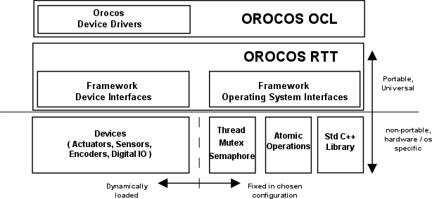
The OS directory contains C++ classes to access Operating System functionality, like creating threads or signaling semaphores. Two kinds of subdirectories are used: the CPU architecture (i386, powerpc, x86_64) and the Operating System (gnulinux, xenomai, lxrt), or target.
RTAI/LXRT is an environment that allows user programs to run with real-time determinism next to the normal programs. The advantage is that the real-time application can use normal system libraries for its functioning, like showing a graphical user interface.
An introduction to RTAI/LXRT can be found in the Porting to LXRT HOWTO, which is a must-read if you don't know what LXRT is.
The common rule when using LXRT is that any user space (GNU/Linux) library can be used and any header included as long as their non-real-time functions are not called from within a hard real-time thread. Specifically, this means that all the RTAI (and Orocos) OS functions, but not the native Linux ones, may be called from within a hard real-time thread. Fortunately these system calls can be done from a not hard real-time thread within the same program.
The OS directory is the only part of the Real-Time Toolkit that needs to be ported to other Operating Systems or processor architectures in case the target supports Standard C++. The os directory contains code common to all OSes. The oro_arch directories contain the architecture dependent headers (for example atomic counters and compare-and-swap ).
In order to start your port, look at the fosi_interface.h
and fosi_internal_interface.hpp files in
the os directory. These two files list the C/C++ function
signatures of all to be ported functions in order to support
a new Operating System. The main categories are: time reading, mutexes,
semaphores and threads.
The easiest way to port Orocos to another operating system,
is to copy the gnulinux directory into a new directory and start
modifying the functions to match those in your OS.
The following table gives a short overview of the available headers in the os directory.
Table 7.1. Header Files
| Library | Which file to include | Remarks |
|---|---|---|
| OS functionality | rtt/os/fosi.h | Include this file if you want to make system calls to the underlying operating system ( LXRT, GNU/Linux ) . |
| OS Abstraction classes | Mutex.hpp, MutexLock.hpp, Semaphore.hpp, PeriodicThread.hpp, SingleThread.hpp, main.h | The available C++ OS primitives. main.h is required to be included in your ORO_main() program file. |
All tasks in the real-time system have to be performed by some
thread. The OS abstraction expects an int
ORO_main(int argc, char** argv) function (which
the user has written) and will call that after all system
initialisation has been done. Inside ORO_main() the user
may expect that the system is properly set up and can be used.
The resulting orocos-rtt library will contain the real main()
function which will call the ORO_main() function.
| Important | |
|---|---|
Do not forget to include
|
| Note | |
|---|---|
Using global objects ( or static class
members ) which use the OS functions before ORO_main() is
entered (because they are constructed before main() ), can
come into conflict with an uninitialised system. It is
therefor advised not to use static global objects which use
the OS primitives. |
An Orocos thread by the
Thread class. The most
common operations are start(),
stop() and setting the periodicity.
What is executed is defined in an user object which
implements the
RunnableInterface. It
contains three methods :
initialize(),
step() and
finalize(). You can inherit from
this interface to implement your own functionality. In
initialize(), you put the code that has to be executed once
when the component is start()'ed. In step(), you put the
instructions that must be executed periodically. In
finalize(), you put the instructions that must be executed
right after the last step() when the component is stop()'ed.
However, you are encouraged NOT to use the OS classes! The Core Primitives use these classes as a basis to provide a more fundamental activity-based (as opposite to thread based) execution mechanism which will insert your periodic activities in a periodic thread.
Common uses of periodic threads are :
Running periodic control tasks.
Fetching periodic progress reports.
Running the CoreLib periodic tasks.
A special function is forseen when the Thread executes non periodically (ie getPeriod() == 0): loop(), which is executed instead of step and in which it is allowed to not return (for a long time).
The user himself is responsible for providing a mechanism to
return from the loop() function. The Thread expects
this mechanism to be implemented in the
breakLoop() function, which must return
true if the loop() function could be signaled to
return. Thread will call breakLoop() in its stop()
method if loop() is still being executed and, if successful,
will wait until loop() returns. The
Thread::isRunning() function can
be used to check if loop() is being executed or not.
| Note | |
|---|---|
The Activity provides a better integrated implementation for SingleThread and should be favourably used. |
Common uses of non periodic threads are :
Listening for data on a network socket.
Reading a file or files from hard-disk.
Waiting for user input.
Execute a lengthy calculation.
React to asynchronous events.
The Orocos thread priorities are set during thread
construction time and can be changed later on with
setPriority. Priorities are integer
numbers which are passed directly to the underlying OS. One
can use priorities portably by using the
LowestPriority,
HighestPriority and
IncreasePriority variables
which are defined for each OS.
OSes that support multiple schedulers can use the
setScheduler function to influence
the scheduling policy of a given thread. Orocos guarantees
that the ORO_SCHED_RT and
ORO_SCHED_OTHER variables are
defined and can be used portably. The former `hints'
a real-time scheduling policy, while the latter `hints'
a not real-time scheduling policy. Each OS may define
additional variables which map more appropriately to
its scheduler policies. When only one scheduling policy
is available, both variables map to the same scheduler.
You can configure the OS layer at compilation time using CMake to report thread execution as block-waves on the parallel port or any other digital output device. Monitoring through the parallel port requires that a parallel port Device Driver is installed, and for Linux based OSes, that you execute the Orocos program as root.
If the Logger is active, it will log the mapping of
Threads to the device's output pins to the orocos.log
file. Just before step() is entered, the pin will be set
high, and when step() is left, the pin is set low again.
From within any RTT activity function, you may then additionally use the
ThreadScope driver as such :
  DigitalOutInterface* pp = DigitalOutInterface::nameserver.getObject("ThreadScope");
if ( pp )
    pp->setBit( this->getTask()->thread()->threadNumber(), value );
which sets the corresponding bit to a boolean value. The main thread claims pin zero, the other pins are assigned incrementally as each new Orocos thread is created.
Orocos OS only provides a few synchronisation primitives, mainly for guarding critical sections.
There are two kinds of Mutexes : Mutex
and MutexRecursive. To lock a mutex, it
has a method lock(), to unlock, the method is unlock() and to
try to lock, it is trylock().
A lock() and trylock() on a recursive mutex from the same
thread will always succeed, otherwise, it blocks.
For ease of use, there is a MutexLock which gets a Mutex as argument in the constructor. As long as the MutexLock object exists, the given Mutex is locked. This is called a scoped lock.
Example 7.1. Locking a Mutex
The first listing shows a complete lock over a function :
  Mutex m;
  void foo() {
     int i;
     MutexLock lock(m);
     // m is locked.
     // ...
  } // when leaving foo(), m is unlocked.
Any scope is valid, so if the critical section is smaller than the size of the function, you can :
  Mutex m;
  void bar() {
     int i;
     // non critical section
     {
        MutexLock lock(m);
        // m is locked.
        // critical section
     } //  m is unlocked.
     // non critical section
     //...
  }
Orocos provides a C++ semaphore abstraction class Semaphore. It is used mainly for non periodic, blocking tasks or threads. The higher level Event implementation in CoreLib can be used for thread safe signalling and data exchange in periodic tasks.
  Semaphore sem(0); // initial value is zero.
  void foo() {
     // Wait on sem, decrement value (blocking ):
     sem.wait()
     // awake : another thread did signal().

     // Signal sem, increment value (non blocking):
     sem.signal();

     // try wait on sem (non blocking):
     bool result = sem.trywait();
     if (result == false ) {
         // sem.value() was zero
     } else {
         // sem.value() was non-zero and is now decremented.
     }
  }
Table of Contents
This document provides a short introduction to the Orocos Hardware Device Interface definitions. These are a collection of classes making abstraction of interacting with hardware components.
Designing portable software which should interact with hardware is very hard. Some efforts, like Comedi propose a generic interface to communicate with a certain kind of hardware (mainly analog/digital IO). This allows us to change hardware and still use the same code to communicate with it. Therefore, we aim at supporting every Comedi supported card. We invite you to help us writing a C++ wrapper for this API and port comedilib (which adds more functionality) to the real-time kernels.
We do not want to force people into using Comedi, and most of us have home written device drivers. To allow total implementation independence, we are writing C++ device interfaces which just defines which functionalities a generic device driver should implement. It is up to the developers to wrap their C device driver into a class which implements this interface. You can find an example of this in the devices package. This package only contains the interface header files. Other packages should always point to these interface files and never to the real drivers actually used. It is up to the application writer to decide which driver will actually be used.
The Device Interface can be structured in two major parts : physical device interfaces and logical device interfaces. Physical device interfaces can be subdivided in four basic interfaces: AnalogInput, AnalogOutput, DigitalInput, DigitalOutput. Analog devices are addressed with a channel as parameter and write a ranged value, while digital devices are addressed with a bit number as parameter and a true/false value.
Logical device interfaces represent the entities humans like to work with: a drive, a sensor, an encoder, etc. They put semantics on top of the physical interfaces they use underneath. You just want to know the position of a positional encoder in radians for example. Often, the physical layer is device dependent (and thus non-portable) while the logical layer is device independent.
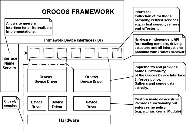
An example of the
interactions between the logical and the physical layer is the
logical encoder with its physical counting card. An encoder is
a physical device keeping track of the position of an axis of
a robot or machine. The programmer wishes to use the encoder
as a sensor and just asks for the current position. Thus a
logical encoder might choose to implement the
SensorInterface which provides
a read(DataType & ) function.
Upon construction of the logical sensor, we supply the real
device driver as a parameter. This device driver implements
for example AnalogInInterface
which provides read(DataType & data, unsigned
int chan) and allows to read the position of a
certain encoder of that particular card.
The most common used interfaces for machine control
are already implemented and tested on multiple setups.
All the Device Interface classes reside in the
RTT namespace.
There are several classes for representing different kinds of IO. Currently there are:
Table 8.1. Physical IO Classes
| Interface | Description |
|---|---|
| AnalogInInterface | Reading analog input channels |
| AnalogOutInterface | Writing analog output channels |
| DigitalInInterface | Reading digital bits |
| DigitalOutInterface | Writing digital bits |
| CounterInterface | Not implemented yet |
| EncoderInterface | A position/turn encoder |
From a logical point of view, the generic SensorInterface<T> is an easy to use abstraction for reading any kind of data of type T.
You need to look in the Orocos Component Library
for implementations of the Device Interface.
Examples are Axis and
AnalogDrive.
The methods in each interface are well documented and porting existing drivers (which mostly have a C API) to these should be quite straight forward. It is the intention that the developer writes a class that inherits from one or more interfaces and implements the corresponding methods. Logical Devices can then use these implementations to provide higher level functionalities.
Name Serving is introduced in the Orocos CoreLib documentation.
The Device Interface provides name serving on interface level. This means that one can ask a certain interface by which objects it is implemented and retrieve the desired instance. No type-casting whatsoever is needed for this operation. For now, only the physical device layer can be queried for entities, since logical device drivers are typically instantiated where needed, given an earlier loaded physical device driver.
Example 8.1, “Using the name service” shows how one could query the DigitalOutInterface.
Example 8.1. Using the name service
  FancyCard* fc = new FancyCard("CardName"); // FancyCard implements DigitalOutInterface

  // Elsewhere in your program:
  bool value = true;
  DigitalOutInterface* card = DigitalOutInterface::nameserver.getObject("CardName");
  if (card)
      card->setBit(0, value);    // Set output bit to 'true'.